OPEN ACCESS
This paper uses the multi-material ALE finite element method and the penalty function coupling method to analyze the effects of the three container shapes of cylindrical, truncated cone and drum on the impact response of flexible fluid-filled containers when the volume is constant but the liquid storage amounts are different. For containers of all three shapes, the maximum principal impact stress of the shape increases with an increase in the liquid storage amount. The maximum principal impact stress of the drum-shaped container is the smallest, that of the truncated cone-shaped container is the largest, and the response time of the maximum principal impact stress of the cylindrical container is the shortest.
Flexible Fluid-Filled Container, Shape, Impact Response, Ale Method, Liquid-Solid Coupling
With the wide use of flexible fluid-filled containers in storage and transportation, water conservancy, aerospace and other fields, the impact response of flexible fluid-filled containers has also drawn the attention of a great number of researchers. The impact of flexible fluid-filled containers is not just a matter of structural mechanics, but rather is a nonlinear, complex liquid-solid coupling problem involving large deformations. Impact dynamic analysis must therefore consider not only the deformation of the flexible container, but also the effects of moving liquid loads on the container.
M.Anghileri [1] et al. used a variety of numberical methods to simulate the process where a liquid-filled container is dropped onto the ground and compared the data with the test results, and in the end achieved satisfactory results. Reed P E [2] analyzed the dropping process of water-filled plastic containers and built an equivalent mass-spring model to predict the characteristic pulse time and pressure distribution on the container wall. Cao et al. [3] studied the interactions between the container and the fluid using the penalty function, and the results showed that the dynamic stress and deformation of a flexible liquid-filled container are proportional to the drop height. Li Zheng [4-6] completed a 3D modeling of the drop impact of a large-deformation in a flexible fluid-filled container. Wang Hui [7-8] used four different numberical methods to simulated the process where a flexible liquid-filled container is dropped onto the ground and compared the advantages and disadvantages of these various methods. Li Qiang [9] completed the numerical simulation and calculation of the drop impact process of liquid storage PET bottles. Zhang Wei-wei [10] simulated and studied the process where flexible fluid-filled containers are dropped into water. Other people also have done some related research [11-12]. The above research has mainly focused on theoretical and numerical methods for determining the impacts on flexible fluid-filled containers, while little research has been conducted on the effects of the shape of the fluid-filled container on the impact response. This paper intends to study the effects of the container shape on the impact response. We used the multi-material ALE (Abitrary Lagrangian-Eulerian) modeling method and the penalty function to carry out a numerical simulation of the impact response process and compared the effects of cylindrical, truncated cone and drum shapes on the impact response of the containers.
In large deformation fluid-solid coupling, the Lagrange method can easily cause distortion in describing the grid cells and makes it impossible to complete the calculation, while the Euler method is likely to cause problems in describing the cells such as increased computation space domain and difficulty in tracking the material contact boundary. ALE description is a kind of motion mode independent of the material and space grid. It introduces a reference domain in addition to the material domain and the space domain and resolves on the reference grid, which avoids the serious deformation of the material under the Lagrange grid and eliminates the complex problems caused by the moving boundary under the Euler grid, providing a good method for solving the liquid-solid coupling problem [13-14]. In the ALE method, a third arbitrary reference coordinate, other than Lagrange and Euler coordinates, is introduced, and the material change rate associated with the reference coordinate can be described with the following equation:
$\frac{\partial f({{X}_{i}},t)}{\partial t}=\frac{\partial f({{x}_{i}},t)}{\partial t}+{{w}_{i}}\frac{\partial f({{x}_{i}},t)}{\partial t}$ (1)
where Xi is the Lagrange coordinate, xi is the Euler coordinate, and wi is the relative velocity between the moving velocity vi under the Lagrange coordinate and the moving velocity ui under the Euler coordinate; i.e., wi=vi-ui. Considering the substitutional relationship between the time derivative of material and the time derivative of the reference geometric configuration, the governing equation of the ALE algorithm governing the Newtonian fluid flow in the fixed domain can be obtained from the following conservation equations:
Mass conservation equation:
$\frac{\partial \rho }{\partial t}=-\rho \frac{\partial {{v}_{i}}}{\partial {{x}_{i}}}-{{w}_{i}}\frac{\partial \rho }{\partial {{x}_{i}}}$ (2)
Momentum conservation equation:
$\rho \frac{\partial {{v}_{i}}}{\partial t}={{\sigma }_{ij,j}}+\rho {{b}_{i}}-\rho {{w}_{i}}\frac{\partial {{v}_{i}}}{\partial {{x}_{j}}}$ (3)
Energy conservation equation:
$\rho \frac{\partial E}{\partial t}={{\sigma }_{ij,j}}{{v}_{i,j}}+\rho {{b}_{i}}{{v}_{i}}-\rho {{w}_{i}}\frac{\partial E}{\partial {{x}_{j}}}$ (4)
where σij is the Cauchy stress tensor, σij=-pδij+μ(vi,j+vj,i); ρ is the density; p is the pressure; μ is the coefficient of kinetic viscosity; δij is the Kronecker function; E is the energy per unit mass; bi is the fluid volume force.
The multi-material ALE description can contain multiple materials in a cell, and by tracking the boundaries of each material, it exchanges and transports materials between the corresponding cell, but it needs to effectively track the interfaces of each material. In this paper, we use the VOF (Volume of Fluid) method to track the locations of the material interfaces. This method determines the material interfaces using the function of material volume ratio in an ALE cell, rather than by tracking the movement of particles on the material surface. To solve the multi-material ALE equation, we use the separator splitting technique; that is, dividing the calculation at each step into two stages. First, we perform the Lagrange process, where the grid moves with the material. In this process, the equilibrium equations for the calculation speed and the internal energy variation caused by internal and external forces are as follows:
$\rho \frac{\partial {{v}_{\text{i}}}}{\partial t}={{\sigma }_{ij,j}}+\rho {{b}_{i}}$ (5)
$\rho \frac{\partial E}{\partial t}={{\sigma }_{ij}}{{v}_{i,j}}+\rho {{b}_{i}}{{v}_{i}}$ (6)
In the Lagrange process of calculation, as there is no material flowing across the cell boundary, the mass automatically remains conserved. The second stage of calculation, referred to as the convective term, calculates the mass transport, internal energy, and momentum across the cell boundary, which can be regarded as remapping the displacement grid of the Lagrange process back to its original position or any other position.
Hourglass viscosity is used to control the zero energy mode of the grid. Impact viscosity with linear and quadratic terms is used to obtain the shock wave. To this end, the pressure term is added into the energy equation (the second one listed among the equilibrium equations). The central difference method is used to solve the equation based on time increment using the time-explicit method. The second-order Van Leer method is used to calculate the convective term. In this paper, both the simple average and equipotential average methods are used to calculate the smoothness of the grid.
3.1 Numerical simulation
Based on the multi-material ALE finite element method, we use the explicit finite element software LS-DYNA to carry out the numerical simulation. We built a finite element model according to the actual size of a cylindrical flexible fluid-filled container and the experimental process. The model consists of a cylindrical flexible container, the water and air in the container and a concrete floor. The flexible fluid-filled container is modeled using the LagrangianBelytschko-Tsay (B-T) membrane element, which is a super-elastic material model. The water and air in the container are described with the hexahedral element and the null material model based on the multi-material ALE description. The Gruneisen equation is used as the state equation of water. The pressure is defined as below:
$P=\frac{{{\rho }_{0}}{{C}^{2}}\mu \left[ 1+\left( \text{1-}\frac{{{\gamma }_{\text{0}}}}{\text{2}} \right)\mu \text{-}\frac{\alpha }{\text{2}}{{\mu }^{\text{2}}} \right]}{{{\left[ \text{1-}\left( {{S}_{1}}-1 \right)\mu -{{S}_{2}}\frac{{{\mu }^{2}}}{\mu +1}-{{S}_{3}}\frac{{{\mu }^{3}}}{{{\left( \mu +1 \right)}^{2}}} \right]}^{2}}}+\left( {{\gamma }_{0}}+\alpha \mu \right)E$ (7)
where C is the intercept of the us-up (shock wave velocity -particle velocity) curve; S1, S2 and S3 are the slope coefficients of the us-up curve; γ0 is the Gruneisen parameter; α is the first-order volume correction value; E is the intrinsic energy of material; volume rate of change $\mu \text{=}\frac{\rho }{{{\rho }_{\text{0}}}}\text{-1}$, where ρ is the current density and ρ0 is the initial density. The parameters for the material equation of state (EOS) are shown in Table 1. For the air, the linear polynomial state equation is used. The pressure is defined as a function of internal energy of per unit volume, E. The equation is defined as below:
$P\text{=}{{C}_{0}}+{{C}_{1}}\mu +{{C}_{2}}{{\mu }^{2}}+{{C}_{3}}{{\mu }^{3}}+\left( {{C}_{4}}+{{C}_{5}}\mu +{{C}_{6}}{{\mu }^{2}} \right)E$ (8)
where C0, C1, C2, C3, C4, C5 and C6 are constants. The parameters for the material EOS are shown in Table 2. The physical parameters of the concrete floor are shown in Table 3. The structural mechanical properties of the composite material of the outer container wall are the key to the numerical simulation. According to the woven form, the composite material can be regarded as the transversely isotropic material. In this paper, the mechanical properties of the material are calculated by the method proposed in Reference [15], as shown in Table 4.
Table 1. Parameters for Water EOS
|
ρ (g/cm3) |
C(m/s) |
S1 |
S2 |
S3 |
γ0 |
α |
|
0.998 |
1650 |
1.92 |
-0.096 |
0 |
0.35 |
0 |
Table 2. Parameters for Air EOS (g-cm-μs)
|
ρ (g/cm3) |
C0 |
C1 |
C2 |
C3 |
C4 |
C5 |
C6 |
E0 |
|
1.29e-3 |
0 |
0 |
0 |
0 |
0.4 |
0.4 |
0 |
2.5e-06 |
Table 3. Performance parameters of concrete material
|
Density g/cm3 |
Elasticity modulus GPa |
Poisson's ratio |
|
ρ |
E |
ν |
|
2.665 |
40 |
0.3 |
Table 4. Performance Parameters of Flexible Container Shell Material
|
Elasticity modulus GPa |
E1 |
E2 |
E3 |
|
1.535 |
1.535 |
1.070 |
|
|
Shear modulus GPa |
G12 |
G23 |
G13 |
|
0.389 |
0.267 |
0.267 |
|
|
Poisson's ratio |
ν12 |
ν23 |
ν13 |
|
0.163 |
0.379 |
0.379 |
|
|
Yield stress GPa |
σy |
Density g/cm3 |
ρ |
|
0.2 |
1.1 |
A finite element model was built to simulate the process where a flexible fluid-filled container, filled to 50% of liquid storage capacity, falls from a height of 100m and hits the cement floor. This model has a total of 160178 cells and 165344 nodes, and is shown in Figure 1.
Figure 1. Finite element model of the cylindrical fluid-filled container
In case there is air resistance and in order to shorten the calculation time and save resources, the height of 100m is converted to a speed of 40m/s. The ground is treated as a rigid body. Ground base grid cells are fully constrained. The gravitational acceleration is 9.81m/s. The coupling between the container and the liquid and the collision between the container and the ground are realized by the penalty function. The numerical simulation takes into account the effect of the air inside the container. As we mainly analyze the maximum principal stress of the container, we regard the cover as a part of the shell in modeling. To ensure stability of calculation, the time step is subject to the minimum cell size of the model, the number of liquid-solid coupling points is set to 4, and the minimum volume parameter of coupling is set to 0.1.
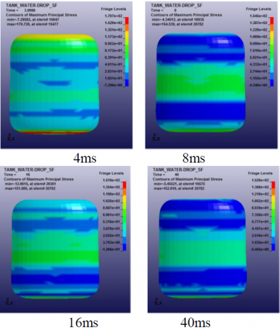
The numerical simulation results are shown in Figure 2 and 3. Figure 2 is the nephogram for the principal stress of the cylindrical container at various moments. Figure 3 shows the form of the liquid in the container at various moments.
Figure 2. Nephogram for the principal stress of the cylindrical container at different moment
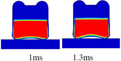
Figure 3. Form of the liquid in the container at different moments
At the moment when the container hits the ground, the container stops moving, but the liquid continues to move downward due to the effect of inertia. The nature of the fluid causes the liquid to move to the surrounding areas at the container bottom and creates impact stress on the container wall. Under the stress, the container is deformed and a portion of the potential energy is converted into deformation energy. The deformed container also has a reaction to the fluid, which forces a change in the fluid velocity and acceleration. This is a liquid-solid coupling process.
It can be seen from Figure 2 and Figure 3 that at the moment of 1.3ms, the stress reaches the maximum value in the whole impact process, and the bottom of the container wall experiences the maximum deformation. Meanwhile, the deformation energy of the container also reaches the maximum value. Then, under its own elastic effect, the container is gradually restored to its original state. At this moment, the fluid moves inward driven by the deformation force of the container, while in the vertical direction, under the rebound effect, the fluid begins to move upward, resulting in a cavity at the bottom and further reducing the pressure. Later, the cavity is gradually closed, and the pressure rises again. As time passes, the fluid continues to move upward and squeezes towards both sides, and with the liquid flowing upward, the upper air is compressed. The water inside the container splashes up and begins to surround the air. With the upper air compressed, its volume is reduced, and the cavity at the bottom continues to expand due to the upward movement of the fluid, and the pressure is reduced.
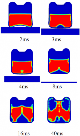
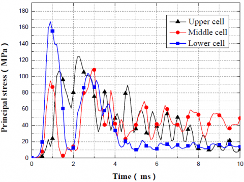
Figure 4 shows the principal stress time-history curves of the three cells selected from the upper, middle, and lower parts in the outer wall of the container. It can be seen that the principal stress of each of the three parts reaches the maximum value in sequence of the lower, upper and middle parts. The lower part has the highest stress value, followed by the upper part and the middle part. This is also consistent with the results of container rebound deformation in the experiment. It can be seen that the maximum principal stress of the lower part of the container occurs before that of the upper part, with an amplitude greater than that of the latter. The maximum principal stress of each of the two cells reaches the peak and then rapidly falls and oscillates at a smaller amplitude, and gradually reaches a steady state.
Figure 4. Principal stress time-history curves of the three cells in the upper, middle and lower parts
3.2 Effectiveness verification of numerical simulation
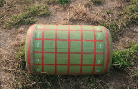
In this paper, we verify the effectiveness of the numerical simulation mainly through experiments. A cylindrical flexible fluid-filled container mainly consists of a container body, a cover and ancillary devices, as shown in Figure 5. It has a height of 430cm and a diameter of 360cm. The body is reinforced with fabric, and the base is made of natural rubber with a thickness of 1.5cm. When the liquid storage amount is 50%, 80% and 100% of capacity respectively, we drop the container from a height of 100m and with a high-speed camera film the dynamic response process of the container after being dropped. Then we process and analyze the data and obtain the relationship between the drop impact velocity and the deformation of the container.
Figure 5. Cylindrical flexible fluid-filled container
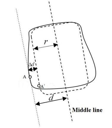
We verify the effectiveness of the numerical simulation results mainly by analyzing whether the relationships between the deformation of the container and the time are consistent in the impact processes respectively in the experiment and numerical simulation. If the numerical simulation is the same as or similar to the experiment result, the numerical simulation results are considered acceptable. Specifically speaking, we select several points on the outer wall of the container, and then analyze whether the displacement variations of the points with time are consistent with those in the simulation to determine the correctness of the simulation. As shown in Figure 6, Δd is the variation in the distance between a point on the outer wall of the container and the center of the container; d is the distance between the point and the center line of the container (cylindrical tank) at different moments during the impact process; r is the instantaneous radius of the cylindrical fluid-filled container contacting the ground; t0 is the moment when the container drops and touches the ground. If the change rule of Δd over time is consistent with the numerical simulation, then we consider the simulation results to be accurate. The expression of Δd is as follows:
$\Delta d=\left\{ \begin{matrix} \text{0}(t={{t}_{0}}) \\ d-r(t>{{t}_{0}}) \\\end{matrix} \right.$
Figure 6. Verification method for the effectiveness of the numerical simulation
Figure 7 shows the comparison between the variations in the distances from the three points in the upper, middle and lower parts to the centerline and the numerical simulation results. It is found that the numerical simulation results deviate a little from the physical experiment results, with the maximum deviation being 6%. This is probably because the numerical simulation model has simplified the process. But if this simulation is used to analyze the impact responses of flexible containers of different shapes, such deviations are still acceptable. It can accurately reflect the actual drop impact process of the container.
Figure 7. Comparison between test results and numerical simulation results
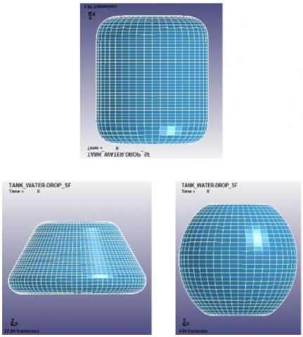
We built the 3D finite element models for truncated cone-shaped and drum-shaped flexible fluid-filled containers respectively so as to compare them with the cylindrical container. The three kinds of containers have the same liquid capacity and are made of the same material, and we assume they have no cover or accessory. Calculation results show that the mass of the three differently-shaped containers with the same volume differs by no more than 9% and that the mass of an empty container accounts for no more than 6% of the total mass of a container containing a liquid storage amount at 50% of capacity. For convenience of comparison, we ignore the response result errors caused by the differences in container mass. The finite element models built, shown in Figure 8, are used to carry out the numerical simulation of the drop impact process of the above three kinds of containers with a liquid storage amount at 50%, 80% and 100% of capacity respectively.
Figure 8. Finite element models for three container shapes
4.1 Comparison of three different container shapes under different liquid storage conditions
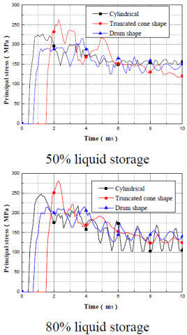
Figure 9. Time-history curves of maximum principal stress elements under different liquid storage conditions
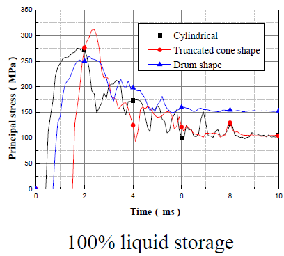
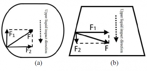
Figure 9 shows the time-history curves of the maximum principal stress elements in the three containers under different liquid storage conditions. It can be seen that regardless of whether the liquid storage amount is at 50%, 80% or 100% of capacity, the maximum impact stress of the drum-shaped container is the smallest, indicating that the drum-shaped container has better resistance to impact than the other two container shapes. This is mainly because in the impact process, the container is deformed under the fluid load and in turn it reacts on the fluid. Figure 10(a) shows the reaction force of the drum-shaped container against the fluid. In this figure, the reaction force F of the container on the fluid is inwardly vertical to the container wall, which can be decomposed into the vertical force F1 and the horizontal force F2. Due to the symmetrical structure of the container, the reaction forces in the horizontal direction cancel each other out, and the component force in the vertical direction can partially offset the vertical impact load from the upper liquid, thereby reducing the impact force on the container. Meanwhile, as the structure of the drum-shaped container upwardly opens up, there is more space for the liquid that is rebounded upwards, reducing the pressure and dispersing the rebound impact pressure. In contrast, the structure of the truncated cone-shaped container is completely different, as shown in Fig. 10 (b). The fluid impact load and the reaction force of the container on the fluid are superposed, increasing the impact force on the container.
Figure 10. Diagram for the reaction force of the container on the fluid
In terms of the response time of the maximum principal stress, whether the liquid storage amount is at 50%, 80% or 100% of capacity, the cylindrical container responds the fastest, the drum-shaped container responds the slowest at the storage amount of 50% and 80% of capacity and the truncated cone-shaped container responds the slowest at the storage amount of 100% of capacity. Such differences in the response time may have something to do with the container shape, a question which merits further studies.
4.2 Comparison of containers of the same shape but under different liquid storage amounts
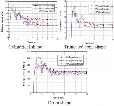
Figure 11. Time-history curves of the maximum principal stress elements in containers of different shapes
Figure 11 shows the stress time-history curves of the maximum principal stress elements in containers of different shapes. It can be seen from the figure that the maximum principal stress of each container increases with an increase in the liquid storage amount, and the maximum principal stress element reaches the stable stress value faster when the storage amount is increased. When the liquid storage amount is at 100% of capacity, the stable stress values of the cylindrical and truncated cone-shaped containers are smaller than those with a liquid storage amount at 50% and 80% of capacity, while that of the drum-shaped container with a liquid storage amount at 100% of capacity is roughly similar to those with a liquid storage amount at 50% and 80% of capacity.
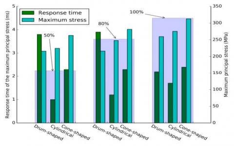
Figure 12. Maximum principal stress and response time by container shape and liquid storage amount
Figure12 shows the maximum principal stress and response time by container shape and liquid storage amount. From Figure 12, we can see that when the liquid storage amount changes from 50% to 80% and 100% of capacity, the maximum principal stress of the containers of different shapes also respond at different speeds. The response rateof the cylindrical container becomes gradually faster, that of the truncated cone-shaped container does not change significantly, and that of the drum-shaped container first gets higher and then rapidly decreases. The maximum stresses of the containers of different shapes also change at different rates. The maximum principal impact stress of the cylindrical container and the truncated cone-shaped container gradually increase with an increase in the liquid storage amount, while that of the drum-shaped container does not change much when the liquid storage amount is at 50% and 80% of capacity. Changes in the maximum principal impact stress amplitudes of the cylindrical and the truncated cone-shaped containers are not significantly different. When the liquid storage amount changes from 50% to 100% of capacity, changes in the maximum principal impact stress amplitudes of the cylindrical, truncated cone-shaped and drum-shaped containers are 50.8MPa, 49.5MPa and 43.4MPa respectively. The question of why the changes for the cylindrical and truncated cone-shaped containers are quite similar merits further studies.
4.3 Position of the maximum principal stress
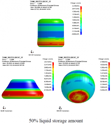
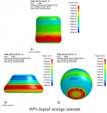
Figure 13. Stress nephogram at the maximum principal stress time by liquid storage amount and container shape
Figure 13 reveals that the position of the maximum principal stress in the cylindrical container basically remains the same, and the distribution range of the maximum principal stress in the cylindrical container takes the shape of "Λ" , and is distributed most widely when the liquid storage amount is 80% of capacity.The position of the maximum principal stress in the truncated cone-shaped container gradually rises vertically with an increase in the liquid storage amount, and the distribution range does not change much.For the drum-shaped container, when the liquid storage amount is at 50% or 80% of capacity, the maximum principal stress is located at the bottom edge of the container, while when the storage amount is at 100% capacity, the maximum stress is in the lower outer part of the container, with the widest distribution.
(1) Under the same liquid storage condition, containers of different shapes have significantly different maximum principal impact stresses and maximum principal stress response times. Under all the three liquid storage amount conditions, the drum-shaped container has the smallest maximum principal stress, and the cylindrical container requires the shortest maximum principal stress response time.
(2) The maximum principal stresses of all the three container shapes increase with an increase in the liquid storage amount, but at different speeds.
(3) In the same container shape, under different liquid storage conditions, the position of the maximum principal stress is different.
[1] Anghileri M., Castelletti L.M.L., Tirelli M. (2005). Fluid–structure interaction of water filled tanks during the impact with the ground, International Journal of Impact Engineering, Vol. 31, No. 3, pp. 235-254. DOI: 10.1016/j.ijimpeng.2003.12.005
[2] Reed P.E., Breedveld G., Lim B.C. (2000). Simulation of the drop impact test for moulded thermoplastic containers, International Journal of Impact Engineering, Vol. 24, No. 2, pp. 133-153. DOI: 10.1016/S0734-743X(99)00148-7
[3] Cao Y., Jin X.L. (2010). Dynamic response of flexible container during the impact with the ground, International Journal of Impact Engineering, Vol. 37, No. 10, pp. 999-1007. DOI: 10.1016/j.ijimpeng.2010.05.001
[4] Li Z., Jin X.L., Shen J., Chen X.D., Guo L. (2007). Simulation on the Large-Scale Vehicle Flexible Fluid-Filled Structure, Journal of Shanghai Jiao Tong University, Vol. 41, No.1, pp. 19-22. DOI: 10.3321/j.issn:1006-2467.2007.01.005
[5] Li Z., Jin X.L., Chen X.D. (2007). Crash Simulation of Flexible Fluid-Filled Container Based on Arbitrary Lagrangian-Eulerian Formulation Method, Journal of Vibration and Shock, Vol. 26, No.8, pp. 72-75. DOI: 10.3969/j.issn.1000-3835.2007.08.018
[6] Li Z., Jin X.L., Chen X.D. (2008). Study on the Parallel Algorithm for the Simulation of Flexible Fluid-filled Container Crash, Journal of Basic Science and Engineering, Vol. 16, No. 4, pp. 588-595. DOI: 10.3969/j.issn.1005-0930.2008.04.015
[7] Wang H., Zhang H.S., Li G.G., Ding J.H. (2009) Numerical Arithmetic Analysis of Fluid-Filled Container During the impact with the ground, Chinese Academic Conference on Mechanics 2009, Zhengzhou, pp. 278.
[8] Wang H., Zhang H.S. (2009). Numerical Simulation of Flexible Fluid-Filled Container during the Impact with Ground, Noise and Vibration Control, Vol. 29, No. 2, pp. 46-50. DOI: 10.3969/j.issn.1006-1355.2009.02.013
[9] Li Q., Liu S.L., Ying G.Y., Zheng S.Y. (2012). Numerical simulation for drop impact of PET bottle considering fluid-structure interaction, Journal of Zhejiang University (Engineering Science), Vol. 46, No. 6, pp. 980-986. DOI: 10.3785/j.issn.1008-973X.2012.06.004
[10] Zhang W.W., Jin X.L., Liu T. (2015) Numerical simulation on water entry of composite flexible fluid reservoir, Chinese Journal of Computational Mechanics, Vol. 32, No. 5, pp. 633-638. DOI: 10.7511/jslx201505009
[11] Luo W., Li Y., Wang Q.H., Li J.L., Liao R.Q., Liu Z.L. (2016). Experimental study of gas liquid two-phase flow for high velocity in inclined medium size tube and verification of pressure calculation methods, International Journal of Heat and Technology , Vol. 34, No. 3, pp. 455-464. DOI: 10.18280/ijht.340315
[12] Wang C., Qin H.D., Liu G., Guo T. (2016). Study on sloshing of liquid tank in large LNG FSRU based on CLSVOF method, International Journal of Heat and Technology, Vol. 34, No. 4, pp. 616-622. DOI: 10.18280/ijht.340410
[13] Nitikitpaiboon C., Bathe K.J. (1993). An arbitrary lagrangian-eulerian velocity potential formulation for fluid-structure interaction, Computers & Structures, Vol. 47, No. 4-5, pp. 871-891. DOI: 10.1016/0045-7949(93)90364-J
[14] Takashi N. (1994). Ale finite element computations of fluid-structure interaction problems, Computer Methods in Applied Mechanics & Engineering, Vol. 112, No. 4, pp. 291-308. DOI: 10.1016/0045-7825(94)90031-0
[15] Li Z. (2008). The research and application on numerical computation method of the flexible fluid-filled container, Ph.D. dissertation, School of Mechanical Engineering, Shanghai Jiao Tong University., Shanghai, China.