OPEN ACCESS
Multi-temperature-level systems enlarge the prospects and degrees of freedom for an effective design and an environment-friendly use of energy. Based on a general thermodynamic model of three-thermal cycles and finite thermal capacity of the heat sources, this paper aims at the analysis and the performance optimization of these systems by considering the influence of irreversibility. Suitable dimensionless parameters for an overall optimization are introduced and their influence on the cycle efficiency is investigated. This approach identifies the limitations imposed to the physical processes by accounting for the inevitable dissipation due to their constrained duration and intensity, and constitutes a general thermodynamic criterion for the optimization of three-thermal irreversible systems. Dependence on the main factors is highlighted in a way that shows how to change them in order to improve the overall efficiency. Under this point of view, the analysis evaluates COP improvements and can be used to perform plant diagnostics, besides predicting the system performance. The use of this criterion is exemplified for the absorption chiller application case.
Three-thermal systems, Irreversibility, Thermodynamic optimization, Efficiency improvement, Dimensionless parameters.
The development of technical solution for an effective use of energy is guided by the formulation of optimization criteria based on the thermodynamic principles. If the sole aim is to ascertain COP at given operating conditions, in fact the use of the first principle of thermodynamics will suffice. On the other hand, since every real process occurring as part of an energy conversion system is associated to an unavoidable degradation of the earliest amount of energy, a thermodynamic optimization criterion should provide a qualitative description, properly identify the limitations imposed to the physical processes by accounting for the inevitable dissipation due to their constrained duration and intensity, point out the most relevant parameters and how to change them in order to improve the performance of that process. In this way, the analysis is intent upon evaluating COP improvements and performing plant diagnostics, not only predicting the system performance. To this objective, an accurate evaluation of irreversibility (or entropy production), namely the use of the second principle of thermodynamics, becomes essential.
Multi-temperature-level systems enlarge the degree of freedom for an effective and environment-friendly use of energy. However, the increased complexity of these devices is often prohibitive with regards to a comprehensive modelling of all the details at play, making the calculation very difficult or impossible, and the physical content obscure. An absorption system, in its simplest arrangement, transfers heat between three temperature levels, but more often between four thermal sources with finite heat capacity [1][2]. Even though the development of vapour compression cycles has limited the implementation field of vapour absorption systems, the absorption cycle still pave the way to sustainable and reliable perspectives. However, given the complexity of the heat and mass transfer phenomena occurring in absorption systems, their optimization is still incomplete and has not leaded to conclusive approaches. A three-thermal sources refrigeration system has been originally modelled as the combined cycle of an endo-reversible two-heat sources engine driving an endo-reversible two-heat sources refrigerator [3], and the effect of finite rate heat transfer towards the surroundings has been considered in a second paper [4]. In addition, [5] applies entropy production analysis with an analytic irreversible thermodynamic model. By applying thermodynamic analysis to absorption chillers [6] have shown the necessity of accounting for internal dissipation, and defined the concept of Process Average Temperature (PAT). As for two thermal sources irreversible refrigerators, [7] use a general irreversible thermodynamic model to obtain an expression of the coefficient of performance accounting for the second principle in a way useful to produce maps of efficiency in terms of meaningful dimensionless parameters.
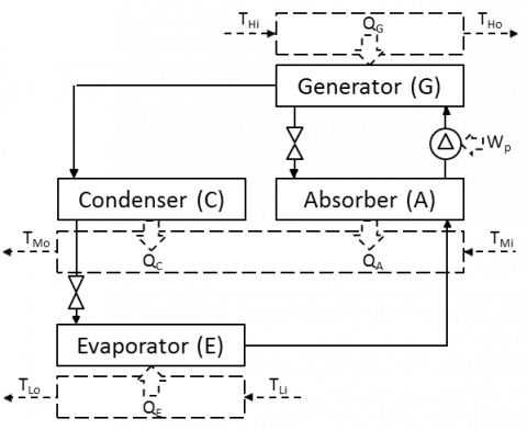
This paper presents a characterization of a three thermal sources inverse thermodynamic cycle that considers the influence of the irreversibilities on the cycle efficiency. Considering a three thermal sources inverse absorption cycle (Fig. 1), the analysis is generalised to include both heat and mass transfer phenomena.
Figure 1. Absorption system schematic
The model is exemplified in a chiller application case. However, except for different temperature ranges and useful effects, absorption chiller, heat pumps or heat transformers are thermodynamically similar units. Thus, the approach can be directly applied to the other system configurations named above.
Steady cyclic-operability is assumed neglecting the effects of potential and kinetic energy of the refrigerant. Since the circulation pump processes saturated liquid solution, its electrical power consumption is disregarded. Furthermore, heat leaks to the surrounding are considered to be ineffective. With the assumptions stated above, the Coefficient of Performance COP is defined as,
$C O P=\frac{Q_{E}}{Q_{G}}$(1)
And the first law states,
$Q_{G}+Q_{E}=Q_{A}+Q_{C}$(2)
Being defined as a state function, entropy variation of the refrigerant performing a closed cycle is null and, if other thermal exchanges are overlooked, internal irreversibilities are transferred outside the cycle to the surroundings through the heat exchangers.
$\Delta S_{F}=\Delta S_{R C}+\left(\Delta S_{R A}+\Delta S_{S A}\right)-\left(\Delta S_{R G}+\Delta S_{S G}\right)-\Delta S_{R E}$(3)
The entropy variation experienced by the pure refrigerant is given by eq. 4.
$\Delta S_{R}=m_{R} \Delta s=m_{R}\left(\int_{i}^{o} \frac{d h}{T}-\int_{i}^{o}\left(\frac{\partial v}{\partial T}\right)_{p} d p\right)$(4)
In general,
$\int_{i}^{o}\left(\frac{\partial v}{\partial T}\right)_{p} d p=l \Delta p$(5)
Where l=bv for a liquid, and l=R/p for a perfect gas [8]. This term accounts for internal irreversibility related to pressure change and includes pressure drops contributions. On the other hand, inside the generator and the absorber the terms related to the entropy variation of the aqueous LiBr solution is expressed as [9],
$\Delta S_{S}=m_{S} \Delta s=$$m_{S}\left\{\int_{T_{i}}^{T_{o}} \frac{1}{T}\left(\frac{\partial h}{\partial T}\right)_{p, X} d T-\int_{p_{i}}^{p_{o}}\left(\frac{\partial v}{\partial T}\right)_{p, X} d p+R\left[\int_{X_{i}}^{X_{0}} \frac{\ln a_{H 2 O}-\ln a_{L B r}}{M_{s o l}} d X\right]\right\}$ (6)
The circulation ratio is introduced according to eq. 7.
$f=\frac{m_{R}}{m_{S}}$(7)
Were the refrigerant mass is related to the concentration difference and the mass of the solution, as in eq. 8.
$m_{R}=\frac{\left(X_{H}-X_{L}\right) m_{S}}{X_{H}}$(8)
Combining equations 3 and 7 with eq. 9, which expresses the thermal power exchanged by the fluid streams of the heat exchangers, and neglecting pressure losses eq. 10 is obtained,
$Q=m \Delta h$(9)
$\Delta S_{F}=$$=\left(Q_{C}+Q_{A}\right) \frac{\left[f \Delta s_{R C}+\left(f \Delta s_{R A}-\Delta s_{S A}\right)\right]}{\left[f \Delta h_{R C}+\left(f \Delta h_{R A}-\Delta h_{s 4}\right)\right]}-Q_{G} \frac{\left(f \Delta s_{R G}-\Delta s_{S G}\right)}{\left(f \Delta h_{R G}-\Delta h_{S G}\right)}-Q_{E} \frac{\Delta s_{R E}}{\Delta h_{R E}}$(10)
Terms of the fractions are evaluated referring to the physical state of the refrigerant and the solution, and the characteristics of the heat exchangers.
Temperature-entropy diagrams are suitable to describe thermodynamic transformations in terms of both the first and second laws. In a previous paper, [10] have presented the use of T-s diagram for aqueous LiBr cycles and a real absorption cycle (from [10]) is represented in Fig. 2. Additional saturation curves at different solution concentrations are meant to extend the depiction to include both the refrigerant (water) and the solution behaviours in absorption cycles.
Figure 2. T-s Diagram of an absorption chiller
Considering an approximate T-s diagram of the traditional absorption refrigeration cycle (the black lines in Fig 2), where condenser and absorber temperature are close, the vapour generation/absorption processes are split into a constant concentration part embodying temperature changes to reach the equilibrium temperature at the generator/absorber, a constant temperature one representing the release/absorption of the heat of absorption, and an isobaric segment to cool down to its saturation temperature the superheated vapour once separated from the solution at its equilibrium. In a first approach, pressure losses are neglected.
$\Delta S_{F}=\frac{\left(Q_{C}+Q_{A}\right)}{T_{A i}} \Theta_{A C}-\frac{Q_{G}}{T_{G i}} \Theta_{G}-\frac{Q_{E}}{T_{E i}} \Theta_{E}$(11)
Where,
$\Theta_{A C}=\frac{T_{A i}\left[f \Delta s_{R C}+\left(f \Delta s_{R A}+\Delta s_{S A}\right)\right]}{\left[f \Delta h_{R C}+\left(f \Delta h_{R A}+\Delta h_{S A}\right)\right]}$
$\Theta_{G}=\frac{T_{G i}\left(f \Delta s_{R G}+\Delta s_{S G}\right)}{\left(f \Delta h_{R G}+\Delta h_{S G}\right)}$
$\Theta_{E}=\frac{T_{E i} \Delta s_{R E}}{\Delta h_{R E}}$(12)
These dimensionless parameters Q depend on temperature, concentration and thermodynamic properties of the refrigerant and the solution within the heat exchangers.
Introducing the definition of heat exchangers effectiveness by [11] kays and London (1954),
$Q_{A C}=\varepsilon_{A C}\left(m c_{p}\right)_{A C \min }\left(T_{A i}-T_{M i}\right)=k_{A C}\left(T_{A i}-T_{M i}\right)=k_{A C} \Delta T_{M}$
$Q_{G}=\varepsilon_{G}\left(m c_{p}\right)_{G \min }\left(T_{H i}-T_{G i}\right)=k_{G}\left(T_{H i}-T_{G i}\right)=k_{G} \Delta T_{H}$
$Q_{E}=\varepsilon_{E}\left(m c_{p}\right)_{E \min }\left(T_{L i}-T_{E i}\right)=k_{E}\left(T_{L i}-T_{E i}\right)=k_{E} \Delta T_{L}$(13)
Accordingly, the expression of the entropy variation becomes,
$\Delta S_{F}=\frac{k_{A C} \Delta T_{M} \Theta_{A C}}{T_{A i}}-\frac{k_{G} \Delta T_{H} \Theta_{G}}{T_{G i}}-\frac{k_{E} \Delta T_{L} \Theta_{E}}{T_{E i}}$(14)
Using the parameters tH, tM and tL
$t_{H}=\frac{\Delta T_{H}}{T_{H i}} \rightarrow \frac{\Delta T_{H}}{T_{G i}}=\frac{\Delta T_{H}}{T_{H i}} \frac{T_{H i}}{T_{H i}-\Delta T_{H}}=\frac{t_{H}}{1-t_{H}}$
$t_{M}=\frac{\Delta T_{M}}{T_{M i}} \rightarrow \frac{\Delta T_{M}}{T_{A i}}=\frac{\Delta T_{m}}{T_{M i}} \frac{T_{M i}}{T_{M i}+\Delta T_{M}}=\frac{t_{M}}{1+t_{M}}$
$t_{L}=\frac{\Delta T_{L}}{T_{L i}} \rightarrow \frac{\Delta T_{L}}{T_{E i}}=\frac{\Delta T_{L}}{T_{L i}} \frac{T_{L i}}{T_{L i}-\Delta T_{L}}=\frac{t_{L}}{1-t_{L}}$(15)
A dimensionless expression is obtained.
$G=\frac{t_{M}}{1+t_{M}} \phi_{\theta^{\prime}}-\frac{t_{H}}{1-t_{H}} \phi_{\theta^{\prime \prime}}-\frac{t_{L}}{1-t_{L}}$(16)
Where,
$\begin{aligned} G=& \frac{\Delta S_{F}}{k_{E} \Theta_{E}} \\ \phi_{\theta^{\prime}} &=\frac{k_{A C} \Theta_{A C}}{k_{E} \Theta_{E}} \\ \phi_{\theta^{\prime \prime}} &=\frac{k_{G} \Theta_{G}}{k_{E} \Theta_{E}} \end{aligned}$ (17)
The COP of the system can be expressed as a function of the dimensionless parameters defined above.
$C O P=\frac{\left|Q_{E}\right|}{\left|Q_{G}\right|}=\frac{\left|Q_{E}\right|}{Q_{A}+Q_{C}-Q_{E}}=\frac{1}{\phi_{t} \frac{t_{M}}{t_{L}}-1}$ (18)
Where,
$\phi_{t}=\frac{k_{A C} T_{M A}}{k_{E} T_{L i}}$ (19)
And using the dimensionless expression of the entropy variation G, it is possible to generalise the absorption chiller efficiency as a function of either tH and tM (eq. 20) or tH and tL (eq. 21).
$C O P=\frac{1}{\phi_{t} \frac{\left[(1-G)\left(1+t_{M}\right)\left(1-t_{H}\right)+t_{M} \phi_{g^{\prime}}\left(1-t_{H}\right)-t_{H} \phi_{g^{*}}\left(1+t_{M}\right)\right]}{t_{M} \phi_{g^{\prime}}\left(1-t_{H}\right)-t_{H} \phi_{g^{*}}\left(1+t_{M}\right)-G\left(1-t_{H}\right)\left(1+t_{M}\right)}-1}$ (20)
$C O P=\frac{1}{\phi_{t} \frac{G\left(1-t_{H}\right)\left(1-t_{L}\right)+t_{H} \phi_{\theta^{\prime}}\left(1-t_{L}\right)+t_{L}\left(1-t_{H}\right)}{\phi_{t}\left[\left(\phi_{\theta^{-}}-G\right)\left(1-t_{H}\right)\left(1-t_{L}\right)-t_{H} \phi_{\theta^{\prime}}\left(1-t_{L}\right)-t_{L}\left(1-t_{H}\right)\right]}-1}$ (21)
The following parametric analysis is based on input experimental data from literature and is intended to explore the results and the feasibility of the present thermodynamic approach. Table 1 contains measured values of the working parameters from real Li/Br absorption chillers. Table 2 shows the values of the dimensionless parameters previously defined and calculated from the equations expressed in appendix A.1.
Table 1. Parameters from literature experimental data
|
|
|
[10] |
[5] |
|
THi |
K |
388.25 |
390.85 |
|
THo |
K |
380.25 |
/ |
|
TGi |
K |
366.83 |
359.31 |
|
TGo |
K |
377.75 |
/ |
|
TMi |
K |
302.15 |
302.55 |
|
TMo |
K |
312.15 |
/ |
|
TCi |
K |
321.45 |
317.45 |
|
TCo |
K |
311.85 |
313.85 |
|
TAi |
K |
325.71 |
330.04 |
|
TAo |
K |
316.54 |
314.58 |
|
TLi |
K |
285.25 |
284.95 |
|
TLo |
K |
280.25 |
280.25 |
|
TEi |
K |
278.25 |
278.75 |
|
TEo |
K |
278.25 |
278.75 |
|
kG |
kW/K |
82.58 |
63.40 |
|
kCA |
kW/K |
140.07 |
103.00 |
|
kE |
kW/K |
203.56 |
86.60 |
|
XH |
|
0.64 |
0.66 |
|
XL |
|
0.60 |
0.58 |
|
COP |
|
0.68 |
0.63 |
Table 2. Dimensionless parameters calculated from literature data
|
|
$\varTheta$E |
$\varTheta$AC |
$\varTheta$G |
tH |
tM |
tL |
$\phi$t |
$\phi$q' |
$\phi$q'' |
G |
COP |
|
[10] |
1.00 |
0.78 |
0.56 |
0.05 |
0.08 |
0.02 |
0.73 |
0.54 |
0.23 |
0.001 |
0.741 |
|
[5] |
1.00 |
0.69 |
0.22 |
0.08 |
0.09 |
0.02 |
0.56 |
0.36 |
0.06 |
0.003 |
0.738 |
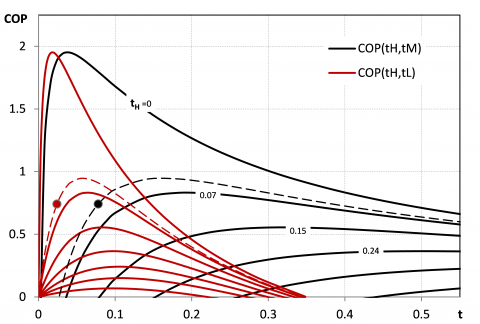
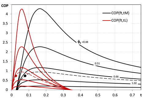
Table 2 makes evidence that the present analysis method tends to slightly overestimate the cycle COP and this could be mainly related to the relatively important impact of heat loss and the assumption of negligible work of the circulation pump. Since the analytical interpretation of equations 20 and 21 is complex, a graphical approach is more convenient and understandable. Figures 3 and 4 represent COP curves as a function of either tL and tM, respectively, for different values of tH or $\phi$t, being other parameters set constant as calculated from [10] in Table 2. These graphs make evidence of the occurrence of a maximal COP. Dashed lines are obtained for the literature value of the secondary variable considered in each graph and the markers represent the operative condition of the real system from [10]. By comparing the actual with the maximum efficiency condition it is possible to perform system diagnostic and show how to improve the overall system efficiency. Fig. 4 shows that the values of the temperature difference parameters maximising the system COP are indipendent from $\phi$t.
Considering the absorption chiller data of [10], given the discrepancy between the experimental values of the temperature difference parameters and the optimal values suggested by the analysis, increasing the temperature difference at low and intermediate temperature heat exchangers, for the same high temperature conditions, or, ceteris paribus, decreasing the temperature difference at the generator, will bring the system closer to the maximum first law efficiency.
Figure 3. COP curves as a function of either tL and tM for different values of tH
Figure 4. COP curves as a function of either tL and tM for different values of $\phi$t
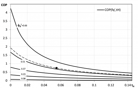
In case the dimensionless parameter representing the irreversibility of the thermal cycle G and the temperature parameter defined for the high temperature thermal source tHare used as variable, COP shows a relentless decreasing trend. when the those are increased (Fig. 5). The same observation is valid with reference to $\phi$q’’ and tH (Fig. 6). While the opposite trend is shown with respect to $\phi$q’ (Fig. 7).
Figure 5. COP curves as a function of tH for different values of G
Figure 6. COP curves as a function of tH for different values of $\phi_{\theta}$’’
Furthermore, if the COP value is fixed, the critical dimensionless parameter for system design can be related as following.
$G=\frac{\left[\frac{t_{L}(1+C O P)}{C O P \phi_{t}}+1\right]\left[t_{H} \phi_{\sigma}\left(t_{L}-1\right)+t_{L}\left(t_{H}-1\right)\right]+\left[\frac{t_{L}(1+C O P)}{C O P \phi_{t}}\right] \phi_{\theta^{\prime}}\left(1-t_{H}\right)\left(1-t_{L}\right)}{\left[\frac{t_{L}(1+C O P)}{C O P \phi_{t}}+1\right]\left(1-t_{H}\right)\left(1-t_{L}\right)}$ (22)
$G=\frac{\left[\frac{(1+C O P)}{t_{M} C O P \phi_{t}}-1\right]\left[t_{M} \phi_{\sigma}\left(1-t_{H}\right)-t_{H} \phi_{\sigma}\left(1+t_{M}\right)\right]-\left(1-t_{H}\right)\left(1+t_{M}\right)}{\left[\frac{(1+C O P)}{t_{M} C O P \phi_{t}}-1\right]\left(1-t_{H}\right)\left(1+t_{M}\right)}$ (23)
Figure 7. COP curves as a function of tH for different values of $\phi_{\theta}$’
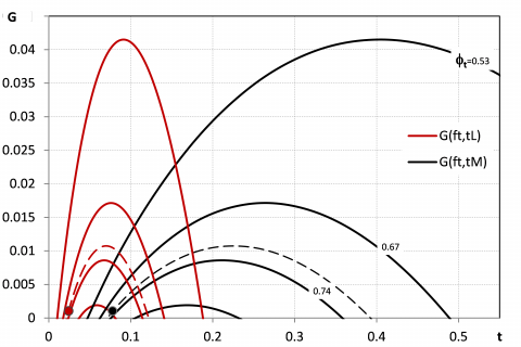
Figures 8 and 9 display the influence of the main dimensionless parameters on the dimensionless function G at constant COP (fixed at the reference value from [10] calculated in table 2) as analitically expressed in eq. 22 and eq. 23.
Figure 8. G curves as a function of either tL and tM for different values of tH
Figure 9. G curves as a function of either tL and tM for different values of $\phi$t
By observing Fig. 8, the dimensionless parameter G, which combines first and second principles of thermodynamics, defines a range limitation of the dimensionless temperature parameters tL and tM for a fixed value of the system COP. These practicable ranges narrow down for higher tH. Moreover, with respect to the same parameters, a maximum value of G can always be associated to defined values of tL and tM, and those values depends on the dimensionless heat conductance parameter $\phi$t (Fig. 9), but not on tH (Fig. 8). The operative condition of the real system described by [10] are plotted in figures 8 and 9, where it is obvious that the system is designed for a low irreversibility operability.
Based on an analytic thermodynamic model for the absorption cycle, this paper presents significant solutions of the key cycle performance by considering the influence of internal irreversibilities due to temperature and concentration variations of the refrigerant. If other thermal exchanges are overlooked, refrigerant irreversibilities are transferred outside the cycle through the heat exchangers to the finite heat capacity sources. In overcoming the limit of the endo-reversible cycle and capturing the fundamental physical phenomena involved, leaving flexibility in generalizing results to other absorption devices, this model provides a predictive and diagnostic tool. Accordingly, suitable dimensionless parameters for an overall system optimization are defined and their influence on best cycle efficiency is investigated in order to perform a first screening of the relevant design and control parameters. In particular, by relating cycle efficiency and entropy variation rates through properly defined dimensionless parameters it is possible to design optimised systems and enhance the performance of existing ones. Namely, if pressure losses in the heat exchangers are negligible, QAC, QG and QE can be calculated once concentration, temperatures and thermodynamic properties of the fluids are available. The dimensionless parameter G stands for the effect of internal irreversibility of the cycle and shows critical impact on the overall performance. By acting on the heat exchangers temperature differences, represented by the corresponding parameters tL, tM and tH, it is possible to maximise the COP of the system. Comparing experimental data from literature with the optimal performance suggested by this analysis possible improvement of the system thermodynamic efficiency are pointed out. Furthermore, the absorption refrigeration cycle model and the thermodynamic analysis can be readily extended to heat pump and heat transformer application cases.
Considering the entropy and enthalpy difference terms related singularly to the transformations constituting the cycle and appearing in eq. 10, the analytical expressions of those variations is presented in the following. As a consequence the dimensionless groups defined in eq. 12 can be developed and calculated, once temperature, concentration and thermodynamic properties of the refrigerant and the solution are defined thorough the cycle. In particular, for the vapour generation process from the refrigerant point of view (1-1’-2 in Fig 2) entropy and enthalpy variations are calculated, respectively, as in eq.s A1 and A2.
$\Delta s_{R G}=c_{p l} \ln \frac{T_{G}}{T_{1}}+\frac{i_{a b s, G}}{T_{G}}$ (A1)
$\Delta h_{R G}=c_{p l}\left(T_{G}-T_{1}\right)+i_{a b s, G}$ (A2)
While, from the solution point of view, the vapour generation process (1-11’-12) is modelled as follows.
$\Delta s_{S G}=c_{p S(p 1, X 1)} \ln \frac{T_{G}}{T_{1}}+R\left[\int_{X_{1}}^{X_{12}} \frac{\ln a_{H 2 O}-\ln a_{L i B r}}{M_{S(p 1, X 1)}} d X\right]$ (A3)
Where, for the estimation of water and lithium-bromide activities a, the calculation procedure presented by [12] is used.
The specific enthalpy variation of the generation and absorption processes also refers to [12], in which the molar enthalpy of pure water and lithium-bromide are combined considering the enthalpy excess, as described by [13].
Similarly, with regard to the entropy variation of the absorption process from the solution standpoint (17-17’-8) eq. A4 is employed.
$\Delta s_{S A}=c_{p S(p 17, X 17)} \ln \frac{T_{A}}{T_{17}}+R\left[\int_{X_{8}}^{X_{17}} \frac{\ln a_{H 2 O}-\ln a_{L i B r}}{M_{S(p 17, X 17)}} d X\right]$ (A4)
And, for the vapour absorption process from the refrigerant point of view (7-7’-8) entropy and enthalpy variations are calculated, respectively, as in eq.s A5 and A6.
$\Delta s_{R A}=c_{p v} \ln \frac{T_{A i}}{T_{7'}}+\frac{i_{a b s, A}}{T_{7'}}$ (A5)
$\Delta h_{R A}=c_{p v}\left(T_{A i}-T_{T^{\prime}}\right)+i_{a b s, A}$ (A6)
Condensation (2-3-4) and evaporation (5-6-7) of the refrigerant are represented by eq.s A7-A10.
$\Delta s_{R C}=\frac{r_{R C}}{T_{C i}}+c_{p l} \ln \frac{T_{C i}}{T_{4}}$ (A7)
$\Delta h_{R C}=r_{R C}+c_{p l}\left(T_{C i}-T_{4}\right)$ (A8)
$\Delta s_{R E}=\frac{\left(1-x_{5}\right) r_{R E}}{T_{E}}$ (A9)
$\Delta h_{R E}=\left(1-x_{5}\right) r_{R E}$ (A10)
a Chemical activity
cp Specific heat [J∙kg-1K-1]
f Circulation ratio
G Entropy parameter
h Specific enthalpy [J∙kg-1]
iabs Specific absorption heat [J∙kg-1]
k Heat exchanger inventory [W∙K-1]
m Flow rate [kg∙s-1]
M Molar mass [kg∙mol-1]
p Pressure [Pa]
Q Heat transfer rate [W]
R Perfect gas constant [J∙kg-1K-1]
r Latent vaporization heat [J∙kg-1]
S Entropy rate [W∙K-1]
s Specific entropy [J∙kg-1K-1]
T Temperature [K]
t Temperature parameter
v Specific volume [m3∙kg-1]
W Mechanical power [W]
X Lithium Bromide concentration
x Vapour quality
Greek symbols
β Volumetric expansion coefficient
$\epsilon$ Heat exchanger efficiency
$\phi$ Heat conductance parameter
$\varTheta$ Entropy parameter of the fluid
Subscript
A absorber
C condenser
E evaporator
F fluid
G generator
H high
H2O water
i inlet
L low
l liquid
LiBr lithium bromide
M intermediate
min minimum
o outlet
p pump
$\theta$ related to $\varTheta$ parameter
R refrigerant
S solution
t related to k parameter
1. Feidt M., “Thermodynamics applied to reverse cycle machines, a review,” International Journal of Refrigeration, 33, 1327-1342, 2010. DOI: 10.1016/j.ijrefrig.2010.07.016.
2. Feidt M., “Evolution of thermodynamic modelling for three and four heat reservoirs reverse cycle machines: A review and new trends,” International Journal of Refrigeration, 36, 8-23, 2013. DOI: 10.1016/j.ijrefrig.2012.08.010.
3. Yan Z., Chen J., “An optimal endoreversible three heat sources refrigerator,” Journal of Applied Physics, 65 (1), 1-4, 1989. DOI: 10.1063/1.342570.
4. Chen J., Yan Z., “Unified description of endoreversible cycles,” Physiscal Review A, 39 (8), 4140-4147, 1989. DOI: 10.1103/PhysRevA.39.4140.
5. Chua H.T., Gordon J.M., Ng K.C., Han Q., “Entropy production analysis and experimental confirmation of absorption systems,” International Journal of Refrigeration 20, 179-190, 1993. DOI: 10.1016/S0140-7007(96)00075-8.
6. Ng K.C., Tu K., Chua H.T., Gordon J.M., Kashiwagi T., “Thermodynamics analysis of absorption chillers: internal dissipation and process average temperature,” Applied Thermal Engineering, 18 (8), 671-682, 1998. DOI: 10.1016/S1359-4311(97)00119-1.
7. Grazzini G., Rocchetti A., “Thermodynamic optimization of irreversible refrigerators,” Energy Conversion and Management, 84, 583-588, 2014. DOI: 10.1016/j.enconman.2014.04.081.
8. Grazzini G., Gori F., “Entropy parameters for heat exchangers design,” Int. J. Heat Mass Transfer, 31, 2547-2554, 1988. DOI: 10.1016/0017-9310(88)90180-9.
9. Lee S.F., Sherif S.A., “Thermodynamic analysis of a lithium bromide/water absorption system for cooling and heating applications,” International Journal of Energy Research, 25, 1019-1031, 2001. DOI: 10.1002/er.738.
10. Tozer R., Syed A., Maidment G., “Extended temperature-entropy (T-s) diagrams for aqueous lithium bromide absorption refrigeration cycles,” International Journal of Refrigeration, 28, 689-697, 2005. DOI: 10.1016/j.ijrefrig.2004.12.010.
11. Kays W., London A.I., Compact Heat Exchangers, MacGraw-Hill, New York, 1964.
12. Palacho-Bereche R., Gonzales R., Nebra S.A., “Exergy calculation of lithium bromide-water solution and its application in the exergetic evaluation of absorption refrigeration systems LiBr-H2O,” International Journal of Energy Research, online library, 2010.
13. Kim D.S., Infante-Ferreira C.A., “A Gibbs energy equation for LiBr aqueous solutions,” International Journal of Refrigeration, 29, 36-46, 2006. DOI: 10.1016/j.ijrefrig.2005.05.006.