OPEN ACCESS
In this paper, a solar tower power plant with a closed Joule-Brayton cycle, of 5 MW rate power, with molten salts thermal storage, located in Seville is presented. The peculiarity of the cycle, using air like fluid work, is to vary, by an auxiliary compressor and a vent valve, the pressure, so that fluid average density, at gas turbine inlet. An adjustment of the mass flow rate, in order to regulate the exit air temperature from the receiver of concentrating solar tower, is obtained. During energy surplus production, the thermal storage energy is loaded. Particular attention is placed to the energy thermal storage, which uses molten salt KCl-MgCl2, suitable for this application due to its high melting temperature, in double tank configuration.
The thermodynamic model of the entire plant was implemented using Thermoflex® software, while, for the concentrating tower, WinDelsol software was used. Using time data relating to the locations, the performance of the entire plant, during a year, has been simulated. Preliminary results show that this plant can achieve relevant benefits in total energy production and equivalent operation hours per year, therefore it is competitive with conventional energy production systems.
Furthermore, a performances estimation with a cost analysis, using a LCOE parametric analysis, has been performed.
Thermal energy storage, concentrating solar power, Closed Joule-Brayton cycle, molten salt, Gas turbine, Solar multiple.
The future of our planet depends heavily on protection of the environment and the expansion of the use of renewable energy [1]. In these years the interest in concentrating solar power tower (CSP) is strongly growing, and it is extending also to Italian areas. Actually, in the world, CSP plants produce around 483.6 MW, and 457 MW are at commercial stage, while other 430 MW are in developing [2]. In previous works [3,4] the use of air as working fluid in solar power plants has already been treated.
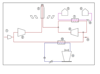
In this paper, a solar thermal power plant, with a Joule-Brayton closed cycle, employing air like fluid work is presented. Figure 1 shows the system, consisting in the CSP plant, a gas turbine as power generation engine, a thermal storage system (TES), cooling subsystem and auxiliary devices.
The CSP plant is composed by the concentrating solar tower and the heliostats field, with a North field configuration, which, through a two axes rotation system, allows conveying the solar radiation at the top of the tower. A cavity volumetric closed receiver, necessary for this plant configuration, has been placed [5].
The power plant consists of a gas turbine of 5 MW peak power, which uses only air. The TES is made up of an air-salt heat exchanger, two storage tanks ("hot" and "cold") operating at temperatures between 790°C and 450°C and a circulation molten salt pump. The thermal storage medium is a mixture of molten salts KCl-MgCl2, whose characteristics are shown in Table 4. Lastly, in the system there are a heat exchanger, which cools down the air temperature at initial conditions of the cycle, an auxiliary compressor and a vent valve, which regulates the pressure, and a cooling tower.
The climate data referring to Seville, for the annual simulations, have been used and they have been extrapolated from TMY3 [6]. The aim of this work is to establish the optimal value of the solar multiple (SM) with the storage capacity (hours at full load) in order to minimize the value of the LCOE.
Annual hourly simulations have been conducted using Thermoflex [7] and varying the hours of thermal storage as well as the SM. The sizing of the heliostat field and the optical efficiency matrix have been obtained by software WinDelsol [8]
Figure 1. Plant scheme: 1. Auxiliary compressor; 2.GT compressor, 3. Solar tower; 4.GT turbine; 5. Cold tank; 6. Hot tank; 7. Storage heat exchanger; 8. Salt pump; 9. Bleed valve; 10. Pre-cooler; 11. Cooling tower.
2.1 Plant description
The described plant used an unfired closed Joule-Brayton cycle. The GT suggested in this paper has a rated power of 5 MW, and the main characteristics are summarized in Table 2.
Table 2. Data using in Joule-Brayton cycle
|
β |
6 |
|
Peak mass flow |
34.6 kg/s |
|
P0 min |
1.01 bar |
|
P0 max |
5.05 bar |
|
P3 max |
30.3 bar |
|
TIT |
800 °C |
|
T0 |
35 °C |
|
Rpm |
3,000 |
|
TOT |
450 °C |
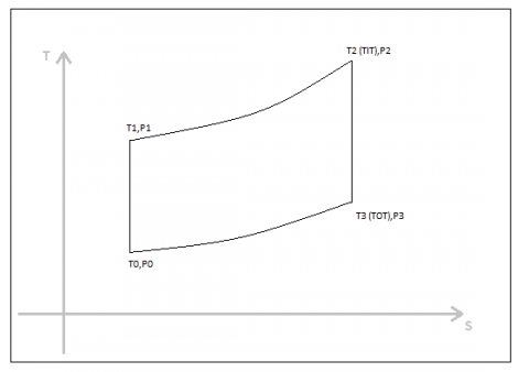
Figure 2. Joule-Brayton cycle refers to table 2
The peculiarity of this system is the possibility of keeping constant the volumetric flow, while varying the mass flow. This is possible through the pressure base variation, obtained by both an auxiliary compressor, placed at GT intake, and a vent valve, located before the pre-cooler. During high values of DNI, the auxiliary compressor sucks up air from the atmosphere, putting air mass in the cycle; vice versa, in the presence of transients, due to clouds or to low values of the DNI, the vent valve bleeds air from the circuit.
The density variation, operated through these auxiliary components, is necessary to ensure the exit air temperature from the receiver at a constant value of 800 ° C. This value is the same of TIT of the GT, when fuel in not used in the cycle, and represents a compromise between the opposite needs off the CSP plant and of the engine system [9].
In this work, the ratios between maximum and minimum temperature and maximum and minimum pressure, characterizing the cycle, have been fixed. The idea is that, we can operate a density variation, through a pressure variation, because components’ volume is fixed. The consequence is a mass variation described by the following low (1):
$\Delta M_{C}=\Delta \rho_{C} V_{C}=\frac{\Delta p_{C}}{R T_{C}} V_{C}$(1)
Consequently, it is possible to have a constant shape cycle (it moves only along S axis in the T-S plane) as well as a constant efficiency, during all operating conditions at different DNI values.
2.2 Storage system description
The storage through TES is well known and it is also advantageous for HGST systems [10]. In this work, the use of TES, without adding fuel in the cycle, has been analyzed. The chosen storage system is a double-tank molten salt type.
The most important parameters are: solidification temperature, vapor pressure, density, heat capacity, viscosity, thermal conductivity and, for the analysis of the heat exchange, the FOM parameter [11].
Through these parameters, the KCl-MgCl2 salt has been selected. It is suitable for this plant configuration, because of its high melting temperatures (> 700 °C), and it is also economically convenient for the ease of retrieval of the raw material.
The following equations show the parameters in function of temperature, used for the simulation in Thermoflex
Table 3. Molten Salt data [12] using in Thermoflex
|
$\rho_{S a l t}=2.05458-0.000474^{*} T\left(^{\circ} C\right)$ |
|
$\mu_{S a l t}=0.0146 * \exp (2230 / \mathrm{T}(K))$ |
|
$C_{p, \text {Salt}}=1.1555+0.0002 * T\left(^{\circ} \mathrm{C}\right)$ |
|
$k_{\text {Salt}}=1.408 * 10^{-4} * \exp (2261.3) / T\left(^{\circ} \mathrm{C}\right)$ |
|
$v_{\text {Salt}}=0.0001408 * \exp (2261.3) / T(K)$ |
While the FOM parameters are defined as [8]:
$F O M_{p f}=\frac{\mu^{0.2}}{\rho^{2} C_{p}^{2.8}}$(2)
$F O M_{a f}=\frac{\mu^{0.2}}{\rho^{0.3} C_{p}^{0.6} k^{0.6}}$(3)
Table 4 shows the characteristics of KCl-MgCl2 molten salt:
Table 4. Characteristic data of KCl-MgCl2 salt
|
Solidification temperature [°C] |
426 |
|
Density [kg/m3] |
1.664 @ 700°C |
|
FOMpf |
5.66 |
|
FOMaf |
39.7 |
|
Molar composition |
68-32 |
|
Thermal conductivity [W/mK] |
0,4 @ 700°C |
|
Heat specific [kJ/kgK] |
1.1555 @ 700°C |
|
Cost €/kg |
0.26 |
2.3 CSP Plant description
The concentrating solar plant is composed by the heliostats field, in north field configuration, the solar tower and the receiver. For the evaluation of SM we assumed that all thermal power source, inlet in the cycle, comes from the CSP plant, because no fuel was used in this kind of system. Therefore in order to design the plant, we estimated the power rate in peak conditions. We took in consideration the air conditions described in Table 2. The specific enthalpy of the air at the end of compression was evaluated by Thermoflex, while the specific enthalpy value at the inlet turbine for hypothesized conditions, was calculated using handbook tables [13]. The peak thermal power required by the Brayton cycle has been evaluated:
$P_{t h, S F}=\dot{m} \times \Delta H$(4)
After a statistical analysis from the TMY data, a design's DNI of 850 W/m2 for the heliostats field has been set. An average field efficiency of ηSF = 0.53 and a heliostat area AHel of 90 m2 have been hypothesized. Therefore by the equation (5) the number of heliostats for each SM configurations has been calculated.
$n_{h e l}=\frac{S M \times P_{r a t e}}{A_{H e l} \times D N I \times \eta_{S F}}$(5)
The results of the equation (5) are shown in Table 5.
Table 5. Heliostats number and reflective area for SM
|
SM |
AT,Hel |
Nel |
|
1 |
44,395 |
493 |
|
1.2 |
53,275 |
593 |
|
1.4 |
62,153 |
691 |
|
1.6 |
71,032 |
798 |
|
1.8 |
79,911 |
888 |
|
2.0 |
88,790 |
987 |
|
2.2 |
97,669 |
1,085 |
|
2.4 |
106,548 |
1,184 |
After the design of the heliostats field, by WinDelsol software, setting the radiative and convective losses, the efficiency matrix, function of azimuth and solar altitude, have been extrapolated. For each SM configuration, and using this matrix, an hourly inlet thermal power in the solar field has been calculated. For example, in Figure 3 the matrix of efficiency for SM = 1 is reported.
Figure 3. Efficiency Matrix of solar field for SM=1; X axis solar altitude, Y axis Azimuth
The availability of hourly power data allows the evaluation of the annual inlet thermal energy, for each configuration. The storage tank volumes, for a ranging time from 2 to 8 hours, using the salt properties listed in Table 4, were calculated. The resulting volumes, and the salt masses, are reported in Table 6.
Table 6. Storage volume and salt mass for different hours of storage.
|
Storage [h] |
Tank volume [m3] |
Salt mass [kg] |
|
1 |
97.3 |
155,749 |
|
2 |
194.7 |
311,499 |
|
3 |
292.0 |
467,249 |
|
4 |
389.4 |
622,999 |
|
5 |
486.7 |
778,748 |
|
6 |
584.0 |
934,498 |
|
7 |
681.0 |
1,090,248 |
|
8 |
778.7 |
1,245,998 |
Due to the variability of the mass flow of the working fluid, that follows the DNI variation, the salt mass flow rates from the tanks change. The values required, to accommodate the different load conditions, have been evaluated.
3.1 Simulation
The annually energy production, for SM=1 configuration, is of 12.50 GWh. Changing the SM, for values ranging from 1.2 to 2.4, the net electric energy produced and plant costs for the different sizes have been evaluated.
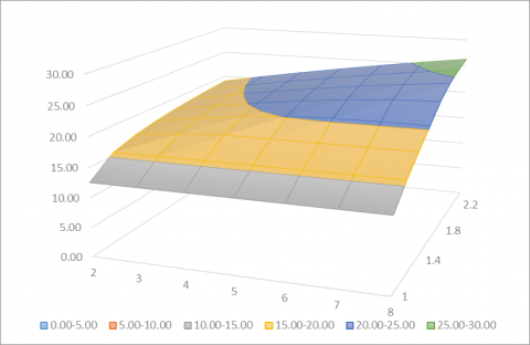
Figure 4 shows the energy production for all configurations (SM and hours of storage); the best configuration can be selected using the minimum value of LCOE.
Figure 4. Energy production [GWh], x axis SM, y axis TES hours, z axis net electric energy
The result appears trivial since the energy production increases with both the hours of storage and the SM. In particular, it increased from 12.50 GWh for SM = 1 to a maximum value of 26.33 GWh for SM = 2.4.
Therefore, the choice of the best configuration is not about only the energy production. It is important to analyze other parameters, like the lost energy for defocusing; this energy cannot produce useful effects, neither for the PB nor for TES, due to their limited size.
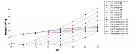
Figure 5 shows the lost and produced energy during a year time.
Figure 5. Lost energy for defocusing and energy produced for different plant configuration.
As shown in Figure 5, it is evident that the increasing of SM causes higher lost energy, so an asymptotic growing trend of the electrical energy production curves is confirmed.
Another parameter, for the choosing of the optimal system configuration is the thermodynamic efficiency, expressed in equation (6):
$\eta_{s y s t e m}=\frac{E_{n e t}}{E_{S F}}$(6)
Table 7. Thermodynamic efficiency of the system for different system configurations
|
Storage [h] |
SM 1 |
SM 1.2 |
SM 1.4 |
SM 1.6 |
SM 1.8 |
SM 2 |
SM 2.2 |
SM 2.4 |
|||||||
|
2 |
0.24 |
0.25 |
0.23 |
0.21 |
0.19 |
0.17 |
0.16 |
0.15 |
|||||||
|
3 |
0.24 |
0.25 |
0.24 |
0.22 |
0.2 |
0.19 |
0.17 |
0.16 |
|||||||
|
4 |
0.24 |
0.25 |
0.24 |
0.23 |
0.21 |
0.2 |
0.18 |
0.17 |
|||||||
|
5 |
0.24 |
0.25 |
0.24 |
0.24 |
0.22 |
0.21 |
0.19 |
0.18 |
|||||||
|
6 |
0.24 |
0.25 |
0.24 |
0.24 |
0.23 |
0.22 |
0.20 |
0.19 |
|||||||
|
7 |
0.24 |
0.25 |
0.24 |
0.24 |
0.24 |
0.23 |
0.21 |
0.20 |
|||||||
|
8 |
0.24 |
0.25 |
0.24 |
0.24 |
0.24 |
0.23 |
0.22 |
0.21 |
|||||||
The data analysis obtained by the equation (6), shows how the best configuration is SM = 1.2, for all the storage capacities. However, the most important parameter about evaluation of the best convenient configuration plant is LCOE, calculated in this work as shown in equation (7):
$LCOE=\frac{\alpha \times {{C}_{inv}}+{{C}_{ma\operatorname{int}}}+{{C}_{fuel}}}{{{E}_{net}}}$ (7)
For the LCOE analysis, the cost values shown in table 8, 9 have been utilized.
Table 8. Investment cost [M USD] for different plant configuration; x axis hours storage, y axis SM
|
Storage [h] |
2 |
3 |
4 |
5 |
6 |
7 |
8 |
|
SM 1.0 |
21.08 |
21.08 |
21.08 |
21.08 |
21.08 |
21.08 |
21.08 |
|
SM 1.2 |
23.78 |
23.96 |
24.15 |
24.33 |
24.52 |
24.70 |
24.89 |
|
SM 1.4 |
26.11 |
26.29 |
26.48 |
26.66 |
26.85 |
27.03 |
27.22 |
|
SM 1.6 |
28.44 |
28.62 |
28.81 |
28.99 |
29.18 |
29.36 |
29.55 |
|
SM 1.8 |
30.77 |
30.95 |
31.14 |
31.32 |
31.51 |
31.69 |
31.88 |
|
SM 2.0 |
33.10 |
33.28 |
33.47 |
33.65 |
33.84 |
34.02 |
34.21 |
|
SM 2.2 |
35.43 |
35.61 |
35.80 |
35.98 |
36.17 |
36.35 |
36.54 |
|
SM 2.4 |
37.76 |
37.94 |
38.13 |
38.31 |
38.50 |
38.68 |
38.87 |
Table 9. Unit cost using in the economic analysis [14][15][16] [17][18]
|
GT cost |
637 |
USD/kW |
|
Heliostats field |
200 |
USD/m2 |
|
Tower and receiver |
200 |
USD/kWth |
|
O&M |
325,000 |
USD |
|
Indirect Cost |
620,8470 |
USD |
|
Storage Cost |
7.1 |
USD/kWhth |
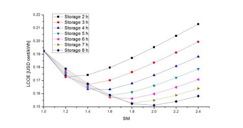
The results of the LCOE analysis are shown in Figure 6.
Figure 6. LCOE analysis for different SM and hour storage
In figure 6 it is possible to note that the minimum value is obtained for SM = 2.0 and 8 hours of storage capacity. In this configuration, the LCOE value is 15.1 ¢$ / kWh.
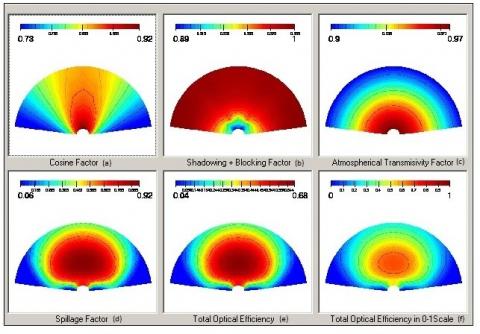
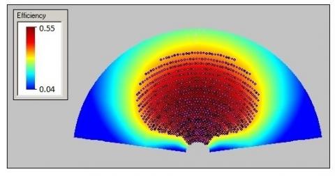
The LCOE analysis parameter shows that the best system configuration is for SM = 2.0. The result is a compromise deriving from the objectives of: system performance, number of working hours, energy lost for defocusing of the heliostats and production of useful energy. A detailed analysis for this CSP plant configuration, obtained from WinDelsol, will be explained. Figure 7 shows the losses in the heliostats field [5]. In particular, diagram (a) shows the cosine factor, varying in the range from 0.78 to 0.92; diagram (b) is related to shadowing and blocking coefficient that ranges between 0.89 and 1. In diagram (c) we can observe the losses for atmospheric transmissivity and exhibits values between 0.9-0.97. Diagram (d) exposes the spillage coefficient, with values between 0.06 and 0.92; the total optical efficiency, lying between 0.04 and 0.68, is shown in diagram (e). Finally, in diagram (f), the same total optical efficiency is plotted in a 0-1 scale. Figure 8 shows the coordinates of the individual heliostats of the best configuration analyzed, where all losses are included, being in total between 0.04 and 0.55.
Figure 7. Field loss
Figure 8. Field layout with all losses
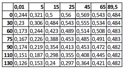
Figure 9. Solar field efficiency matrix for SM = 2.0; X axis solar altitude, y axis azimuth.
The average efficiency obtained, ηSF, is 0.53, according to the assumptions made in the preliminary treatment, while the thermal power incident on the heliostat face is of 80.08 MWth. The height of the tower, calculated by the software, is 100 meters. Figure 9 shows the efficiency matrix of the actual solar field configuration.
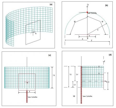
The following figure 10 shows, the size of the receiver, general view (8.a) top view (8.b), side (8.c) and front (8.d), while figure 11 shows the solar flux incident on the receiver.
Figure 10. Complete receiver view (a), above (b), front (c), lateral (d)
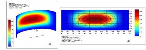
Figure 11. Map receiver incident radiant flux, 3D (a), 2D (b)
The gross power incident on the receiver is of 43.16 MW while the receiver efficiency is 95%.
A technical and an economic analysis for a CSP plant with GT and TES have been conducted. The pressure control system allows to achieve consistent performance, in different operating conditions, without fuel consumption. The use of the mixture of molten salts KCl-MgCl2 is very innovative for the high melting temperatures and for low specific costs, which allows using effectively with the power system proposed. The use of the storage has then allowed to increase the capacity factor of the plant, as well as the operation hours, in the same way as the current solar power systems. The trend of the economic analysis, founded on LCOE method, confirms how the unit cost of energy produced by the plant configuration here presented is similar to the hybrid CSP plants in commercially stage [15]. In conclusion, the study of the utilization of the solar field, with tower, receiver and storage system, provides a very attractive value of LCOE of 15.1 ¢$/kWh, in a solar power plant characterized by SM= 2.0 with a storage having 8 hours capacity. This solution has a value of CF of 55.95%, which is not far from of CF values achieved by typical commercial plants, and higher than the photovoltaic system ones. Considering that this LCOE result was obtained without accounting any incentives, hopefully this technology soon will achieve higher levels of competitiveness in the world energy market.
|
PB DNI CSP TES GT |
Power Block Direct normal irradiance [W/m2] Concentrating solar power Thermal energy storage Gas turbine |
||
|
LCOE |
Levelized cost of electricity [c$/kWh] |
||
|
SM β |
Solar multiple Pressure ratio |
||
|
TIT |
Temperature inlet turbine [°C] |
||
|
ΔH |
Enthalpy variation [kJ/kg] |
||
|
Prate |
Power rate [W] |
||
|
AHel |
Heliostat area [m2/Heliostat] |
||
|
ηSF |
Solar field collector efficiency |
||
|
ηsystem ρSalt μSalt νSalt Cp FOMpf FOMaf ESF Enet Cinv Cmaint CFuel α CF ΔMc Δρc Vc ΔPc R Tc AT,Hel Nel m Pth,SF TOT HSGT |
Thermodynamic system efficiency Molten salt density [kg/m3] Molten salt dynamic viscosity [10-4 Pa Sec] Molten salt cinematic viscosity [m2/Sec] Specific heat at constant pressure [kJ/kg°C] Figure of merit devices P-F [MB2/sec/$] Figure of merit devices A-F [MB2/sec/$] Annual solar field energy [GWh] Net energy production by system [GWh] Investment cost [USD] Maintenance cost [USD] Fuel cost [USD] = 0 Payback factor [10] Capacity factor Mass air variation in the cycle [kg] Density air variation in the cycle Mass air volume of the cycle [m3] Pressure air variation in the cycle [bar] Universal gas constant Average air temperature in the cycle [°C] Heliostat total area [m2] Heliostat total number Mass flow [kg/sec] Thermal power of solar field [kWhth] Temperature outlet turbine [°C] Hybrid Solar Gas Turbine |
||
[1] A. Mirandola and E. Lorenzini. (2016, June). Energy, Environment and Climate: From the Past to the Future. International Journal of Heat and Technology, vol. 34, no. 2, pp. 159-164. Available: http://www.iieta.org/sites/default/files/Journals/HTECH/34.2_01.pdf
[2] http://www.cspworld.org/cspworldmap
[3] M. Cucumo, V. Ferraro, D. Kaliakatsos and V. Marinelli (2013). Energy, Environment and Climate: From the Past to the Future. International Journal of Heat and Technology, vol. 31, no. 2, pp.127-134. Available: http://www.iieta.org/sites/default/files/Journals/HTECH/31.2_17.pdf
[4] M. Amelio, V. Ferraro, V. Marinelli and A. Summaria. (2014, April). An evaluation of the performance of an integrated solar combined cycle plant provided with air-linear parabolic collectors. Energy, vol. 69, pp.742-748. DOI: 10.1016/j.energy.2014.03.068.
[5] E.F. Camacho, M.L. Berenguel, F.R. Rubio and D. Martinez, “6.2.2.1 Volumetric receiver”, “Control of Central Receiver Systems” in Control of Solar Energy Systems, 2012 London, England, pp. 224. DOI: 10.1007/978-0-85729-916-1.
[6] S. Wilcox and W. Marion. (2008, May). Users’ Manual for TMY3 Data Sets. National Renewable Energy Laboratory. Golden, USA. [NREL/TP-581-43156]. http://www.nrel.gov
[7] THERMOFLOW package, THERMOFLEX, Fully-Flexible Heat Balance Engineering Software Available e-mail: INFO@THERMOFLOW.COM
[8] WinDelsol 1.0, “Users Guide”.
[9] W.B. Stine, M. Geyer, “Power Cycles for Electricity Generation” in Power from the sun, 2001. http://www.powerfromthesun.net/book.html
[10] B. Grangea, C. Daleta, Q. Falcoza, F. Sirosb, A. Ferrièrea,, “Simulation of a Hybrid Solar Gas-turbine Cycle with Storage Integration”, in SolarPACES 2013 International Conference. (2014). http://www.sciencedirect.com/science/article/pii/S1876610214005785
[11] R. Williams, D. F., Toth L. M., Clarno K. T., “Assessment of candidate molten salt coolants for the Advanced High-Temperature Reactor (AHTR)” ORNL/TM-2006/12 (2006). http://www.osti.gov/bridge
[12] Williams D. F., “Assessment of candidate molten salt coolants for the NGNP/NHI Heat-Transfer Loop” ORNL/TM-2006/69 (2006). http://www.osti.gov/bridge
[13] Chemical Engineers' Handbook, McGraw-Hill, 5th edition, McGraw-Hill Chemical Engineering Series, 1973. DOI: 10.1036/0071422943.
[14] Craig S. Turchi, Garivin A. Heath- (2013, February). Molten salt power tower cost model for the system advisor model (SAM)-NREL (National Renewable Energy Laboraty).
[15] Gregory J. Kolb, Clifford K. Ho, Thomas R. Mancini and Jesse A. Gary, “Power tower technology roadmap and cost reduction plan”, Sandia report, April, 2011.
[16] P. Schwarzbözl, R.Buck, C.Sugarmen,A Ring, Ma.J. Marcos Crespoc, P.Altweggd and J. Enrilee, “Solar gas turbine systems: Design, cost and perspectives,” Solar Power and Chemical Energy Systems (SolarPACES ‘04), October 2006. http://www.sciencedirect.com/science?_ob=ArticleListURL&_method=list&_ArticleListID=-1025454250&_sort=r&_st=13&view=c&md5=a2dff85e0a9ed690876f860105ac0f24&searchtype=a
[17] C. K. Ho, G.J. Kolb, C. Turchi and M. Mehos, “Current and Future Costs for Parabolic Trough and Power Tower Systems in the US Market” (SolarPACES 2010), September 2010. http://www.sciencedirect.com/science?_ob=ArticleListURL&_method=list&_ArticleListID=-1025454250&_sort=r&_st=13&view=c&md5=a2dff85e0a9ed690876f860105ac0f24&searchtype=a
[18] International Renewable Energy Agency, “renewable energy technologies: cost analysis series” Volume 1: Power Sector Issue 2/5 Concentrating Solar Power. June, 2012.