OPEN ACCESS
In this present study, the numerical simulations are performed for an axisymmetric turbulent jet diffusion hydrogen/air flame, by using a hybrid Finite-Volume/Composition PDF-Transport method. This method represents a rational approach for the study of turbulent reacting flows containing signficant turbulence–chemistry interactions. The major attraction of Composition PDF method is that the terms associated with chemical reaction appear in closed form, leaving only molecular mixing and turbulent transport terms to be modeled. The accuracy of Composition PDF model calculations depends on the accurate representation of the chemistry and on the mixing model including the value of the mixing-model constant CΦ (mixing-model constant CΦ is the mechanical to scalar time scale ratio (CΦ =τt/τΦ).There has been considerable development in the past three decades in PDF methods, and reviews can be found in Dopazo and O’Brien [1] and Subramaniam and Pope [2]. The EMST model, which better describes the physical processes of mixing [3], is used here. An algebraic expression obtained from DNS calculation [4] was implemented, in FLUENT code (ANSYS FLUENT 13.0), via a so-called User Defined Function (UDF) to evaluate the time-scale ratio CΦ in each cell during the simulation course.A comparison is performed with experimental measurements of R.S. Barlow [5].Overall, profile predictions of mixture fraction, flame temperature and major species show a good agreement with experimental data.
PDF method, Turbulent diffusion flame, Micro mixing models, Axisymmetric turbulent reacting jet, turbulence modelling.
Turbulent combustion has many applications in both industrial and natural domains. It can be found in energy production, in aeronautics, in combustion chambers, in some natural phenomena of astrophysics and in environment studies concerning gas discharge in the atmosphere. In the study of this important phenomenon, difficulties related to turbulence as Reynolds tensor and transport terms closures are added to difficulties provided from chemical reaction as the closure of the source terms of combustion which are highly nonlinear.
The standard methods for non-reacting flows (RANS, LES) cannot satisfactorily tackle the problem of the strong non-linearity of the chemical source term and often suffer from a poor modeling of the turbulence-chemistry interaction. However, a detailed modeling of this effect is possible for instance by applying PDF methods. They show a high capability for modeling turbulent flames because these methods treat convection and finite rate non-linear chemistry exactly [6], [7]. Only the effect of molecular mixing has to be modeled [23].
PDF transport equation methods integrated within a conventional CFD flow solver represents a rational approach and an efficacy tool for the study of turbulent combustion.In the PDF transport equation, the term describing the mixing of species at the molecular level (micro-mixing) appears in unclosed form and has to be modelled. The micro-mixing is crucial in turbulent combustion, because chemical reactions take place at molecular scales. Different models for the micro-mixing exist and the most used are the EMST and IEM. The mixing-model constant CΦ is assumed to be constant and the standard value is traditionally setto2.0, but different values have also been used in previous PDF calculations. The standard value 2 is based on the local equilibrium betweenproductionanddissipationofvarianceinisotropicturbulence.Previous studies show that PDF model calculations are sensitive to the value of CΦ [8], [9], [10].The mixing-model constant CΦ is not a universal constant but depends on the initial ratio between the turbulence and scalar time scales as well as on the Reynolds number [24].
In the present work we propose a method based on the combination of transport equations solved by RANS-RSM approach and a statistical method which is the calculation of the PDF. A Lagrangian stochastic particle method is used to solve the PDF equation with the velocity field being obtained from a conventional RANS-RSM approach.
The effect of micro-mixing is modeled using EMST model. To evaluate the time-scale ratio CΦ in each cell during the simulation course, a simple algebraic expression obtained from DNS calculation [4] was used and implemented, in FLUENT 13.0 code, via a so-called User Defined Function (UDF).
A detailed kinetic mechanism which includes 23 elementary reactions and 11 reactive species is used to represent a hydrogen-air reaction. Hydrogen combustion attached much attention recently because of the need for a clean alternative energy.
The basic equations for calculating combustion processes in the gas phase are the equations of continuum mechanics. They include the balance equations for mass, momentum, energy and the chemical species. These equations are written in their Favre-averaged form.
$\frac{\partial \overline{\rho}}{\partial t}+\frac{\partial \overline{\rho} \tilde{u}_{i}}{\partial x_{i}}=0$(1)
\(\frac{\partial \bar{\rho }{{{\tilde{u}}}_{i}}}{\partial t}+\frac{\partial \bar{\rho }\text{ }{{{\tilde{u}}}_{i}}{{{\tilde{u}}}_{j}}}{\partial {{x}_{j}}}=-\frac{\partial \bar{p}}{\partial {{x}_{i}}}+\frac{\mathop{\mathop{\partial (\bar{\tau }}_{ij})}_{eff}}{\partial {{x}_{j}}}+\frac{\partial }{\partial {{x}_{j}}}(-\bar{\rho }\text{ }\overset{\text{ }\!\!\tilde{\ }\!\!\text{ }}{\mathop{{{u}_{i}}''{{u}_{j}}''}}\,)\) (2)
\(\frac{\partial \bar{\rho }\tilde{\varphi }}{\partial t}+\frac{\partial \bar{\rho }{{{\tilde{u}}}_{i}}\tilde{\varphi }}{\partial {{x}_{i}}}=-\frac{\partial \mathop{J}_{i}^{\varphi }}{\partial {{x}_{i}}}-\frac{\partial \text{ }}{\partial {{x}_{i}}}(-\bar{\rho }\text{ }\overset{\text{ }\!\!\tilde{\ }\!\!\text{ }}{\mathop{{{u}_{i}}''\mathop{\varphi }^{''}}}\,)-\bar{\rho }\text{ }\mathop{{\tilde{S}}}_{\varphi }\)(3)
With :
$\left(\tau_{i j}\right)_{e f f}$ viscous stress tensor,
\(-\bar{\rho }\text{ }\overset{\text{ }\!\!\tilde{\ }\!\!\text{ }}{\mathop{{{u}_{i}}''\mathop{u}^{''}}}\,\) the Reynolds stress,
\(-\bar{\rho }\text{ }\overset{\text{ }\!\!\tilde{\ }\!\!\text{ }}{\mathop{{{u}_{i}}''\mathop{\varphi }^{''}}}\,\) the turbulent scalar flux,
$\boldsymbol{J}_{i}^{\varphi}$ the molecular scalar flux and
$S_{\Phi}$ the source term.
For a Newtonian fluid the viscous stress tensor contains only simple shear effects and can be written as:
$\left(\tau_{i j}\right)_{e f f}=\mu_{e f f}\left(\frac{\partial \tilde{u}_{i}}{\partial x_{j}}+\frac{\partial \tilde{u}_{j}}{\partial x_{i}}\right)-\frac{2}{3} \delta_{i j} \mu_{e f f} \frac{\partial \tilde{u}_{i}}{\partial x_{i}}$(4)
With large turbulence Reynolds numbers, the molecular effects are negligible in front of the effects due to turbulent agitation.
In addition to the conservation equations (1)-(3), an equation describing the thermodynamic state is needed. This equation is the gas law for multi-component mixtures:
$P=\rho R T \sum_{\alpha=1}^{n} \frac{Y_{\alpha}}{W_{\alpha}}$(5)
The RSM model version, detailed in our former work [3], is use to modeling the turbulence. The RSM has greater potential to give accurate predictions for complex flows.
First, Reynolds tensor is closed using RSM model. Diffusion species flux is given by Fick’s law. Turbulent transport terms are closed using a transport gradient assumption [3].The transport equations of the Reynolds stress are the following:
\(\frac{\partial }{\mathop{\partial \text{ x}}_{\text{k}}}\text{ (}\mathop{\bar{\rho }{ \tilde{u}}}_{\text{k}}\overset{\tilde{\ }}{\mathop{\mathop{\text{u}}_{\text{i}}\mathop{u}_{j}}}\,\text{) }=\text{ }\mathop{{{\tilde{P}}}}_{\text{ij}}\text{ }+\mathop{{{\tilde{D}}}}_{\text{ij}}+\text{ }\mathop{{\tilde{\varphi }}}_{\text{ij}}\text{-}\frac{\text{2}}{\text{3}}\mathop{\delta }_{\text{ij}}\text{ }\bar{\rho }\tilde{\varepsilon }\text{ }\) (6)
The transport equation of the dynamic dissipation is:
\(\frac{\partial }{\mathop{\partial \text{ x}}_{\text{k}}}\text{ ( }\mathop{\bar{\rho }{ \tilde{u}}}_{\text{k}}\text{ }\tilde{\varepsilon }\text{ ) }=\text{ }\mathop{{{\tilde{D}}}}_{\varepsilon }\text{ }+\text{ }\bar{\rho }\text{ }\frac{\mathop{{\tilde{\varepsilon }}}^{2}}{{\tilde{k}}}\text{ }\tilde{\psi }\text{ (}\varepsilon )\)(7)
Modelling of different terms of equations (6)-(7) is detailed in our former work [3].
Different models are used in turbulent combustion modeling. One of the most popular is the joint probability density function (JPDF) approach, which has been successfully applied in modeling of the turbulence-chemistry interaction.
In the literature many different joint PDF models can be found, for example models for the JPDF of composition, for the JPDF of velocity and composition or for the JPDF of velocity, composition and turbulent frequency. In this work, only a JPDF of composition vector is considered.
This is a one-time, one point JPDF which has the main advantage to treat chemical reactions exactly without any modelling assumptions [6]. However, the effect of molecular mixing has to be modelled.
In composition PDF methods physical scalars, including temperature and species concentrations, are treated as independent random variables. The JPDF is then a function of spatial location, time and composition space. Once the joint PDF is obtained at a certain position x and time instant t, the mean value for any function, Q, of these scalars can be evaluated exactly as:
$<\mathrm{Q}(\phi)>=\int_{-\infty}^{\infty} \mathrm{Q}(\psi) \mathrm{f}(\psi ; x, \mathrm{t}) \cdot \mathrm{d} \psi$(8)
where φ is the vector of physical scalars, is the corresponding random variable vector, Q is a function of φ only and f is the joint PDF, which represents the probability density of a compound event φ = ψ. For variable density flows, it is useful to consider the joint composition mass density function (JCMDF) $\mathrm{F}_{\varphi}(\boldsymbol{\psi})=\rho(\boldsymbol{\psi}) f_{\varphi}(\boldsymbol{\psi})$ . Density weighted averages (Favre averages) can be considered:
\({\tilde{Q} (}x\text{, t) }=\text{ }\frac{<\rho \text{ (}x\text{, t) Q (}x\text{, t)}>}{<\rho \text{ (}x\text{, t)}>}\text{ }=\text{ }\frac{\int\limits_{\psi }{<\text{Q (}x\text{, t)}/\psi >\text{) }\mathop{\text{F}}_{\varphi }\text{ (}\psi ;x\text{, t)}\text{.d}\psi }}{\int\limits_{\psi }{\mathop{\text{F}}_{\varphi }\text{ (}\psi ;x\text{, t)}\text{.d}\psi }}\text{ }\) (9)
4.1 Joint composition PDF transport equation
When the joint composition MDF Fφ is considered, the following transport equation is modelled and solved [6]:
\(\begin{align} & \frac{\mathop{\partial \text{ F}}_{\varphi }}{\partial \text{ t}}\text{ }+\text{ }\frac{\mathop{\partial { \tilde{U}}}_{j}\text{ }\mathop{\text{F}}_{\varphi }}{\mathop{\partial \text{ x}}_{\text{j}}}\text{ }+\text{ }\frac{\partial }{\mathop{\partial \psi }_{\alpha }}\text{ (}\mathop{\text{S}}_{\alpha }\text{ (}\psi \text{) }\mathop{\text{F}}_{\varphi }\text{) } \\ & =\text{- }\frac{\partial }{\mathop{\partial \text{ x}}_{\text{i}}}\text{ }\!\![\!\!\text{ }<\mathop{u}_{i}/\psi >\text{) }\mathop{\text{F}}_{\varphi }\text{ }\!\!]\!\!\text{ - }\frac{\partial }{\mathop{\partial \psi }_{\alpha }}\text{ }\!\![\!\!\text{ }\frac{\text{1}}{\rho \text{ (}\psi \text{)}}\text{ }<-\frac{\mathop{\partial \text{ }J}_{j}^{\alpha }}{\mathop{\partial \text{ x}}_{\text{j}}}/\psi >\text{ }\mathop{\text{F}}_{\varphi }\text{ }\!\!]\!\!\text{ } \\ \end{align}\) (10)
where i and α are summation indices in physical space and composition space, respectively; <A/B>is the conditional mean of the event A, given that the event B occurs. The terms in the LHS (appear in closed form) describe, respectively, evolution of probability in time, convection of probability in the physical space with the mean velocity and transport in composition space due to chemical reaction respectively. Terms on the RHS are unclosed. The first term represents the turbulent transport of probability in physical space (turbulent scalar flux) and is commonly modeled using the gradient diffusion hypothesis, the second term describes the transport of probability in composition space due to molecular fluxes and is further referred to as micro-mixing term. To models, IEM [11] and EMST [2] are often used to close this term. The EMST model, which better describes the physical processes of mixing [3], is used here.
4.2 Hybrid solution method
Equation (10) is solved using the consistent hybrid Finite-Volume/Monte Carlo method presented in [12]. The finite volume method solves for the mean velocity $\tilde{U}$ , the turbulence kinetic energy k, the turbulent dissipation rate ε and the mean pressure<P>. These values and the turbulent time scale $t=k / \varepsilon$ are then passed to the Monte Carlo method. In the Monte Carlo method, the particles are moved through the domain by a spatially second order accurate Lagrangian method. The particles evolve due to different processes such as convection, diffusion, mixing and reaction.
For the numerical solution these processes are applied in different, so-called fractional steps [3].
For the reaction step, the EMST model is used.
The standard value of the time-scale ratio CΦ issetto2.0. In the past, it has been shown that simulation results are often sensitive to this model constant CΦ, and different values have been used. Here, a function for CΦ depending on the Taylor micro-scale Reynolds number Reλ is used. This function is obtained from DNS calculation of CΦ which presents the findings of Overholt and Pope’s [4] investigations of passive scalar mixing in homogeneous isotropic stationary turbulence with imposed constant mean scalar gradient. Further support for such a variation of CΦ with Reλ is provided by recent results of Heinz and Roekaerts [13]. This function is given by:
$C_{\Phi}=\frac{C_{\Phi}(\infty)}{1+1.7 C_{\Phi}^{2}(\infty) R e_{\lambda}^{-1}}$(11)
CΦ(∞) = 2.5, is the asymptotic value CΦ. The Reλ number can be written as a function turbulent Reynolds number Ret [11]:
$\operatorname{Re}_{\lambda}=\left(\frac{20}{3} \operatorname{Re}_{t}\right)^{1 / 2}$(12)
With [14]:
$\operatorname{Re}_{t}=\frac{k^{2}}{\varepsilon v}$(13)
Thus:
$\operatorname{Re}_{\lambda}=\left(\frac{20}{3} \frac{k^{2}}{\varepsilon v}\right)^{1 / 2}$(14)
From equations (11) and (14) we can obtain finally, the time-scale ratio CΦ as a function of of turbulent kinetic energyk and turbulent time scale τt = k/ε:
$\mathrm{C}_{\phi}=\frac{2.5}{1+4.12\left(\frac{k}{v} \tau_{t}\right)^{-(1 / 2)}}$(15)
Equation (15) was implemented, in FLUENT code (ANSYS FLUENT 13.0), via a so-called User Defined Function (UDF).
For the simple jet flame calculations, we use a cylindrical coordinate system with the origin at the center of the fuel jet. In the computations, velocity and length are normalized respectively by the centerline velocity at the inlet Uj and the jet radius Rj (for radial evolution) and visible flame length L [15] (for axial evolution). The computational domain and boundary conditionsare detailed in our former work [3].
In this section, the numerical results for mixture fraction, temperature and major chemical species obtained using UDF are presented and compared to the experimental data of R.S. Barlow and al [5]. The experimental data demonstrate that differential diffusion is important only at the first location (x/Lvis=1/8) [18], [19]. The hydrogen air flame studied here is not influenced by buoyancy because of the high values of the Froude number [20], which are about 17,000.
Figure 1shows the axial profiles of mean mixture fraction. The simulation results are found to be in very good agreement with experimental data.
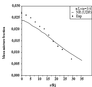
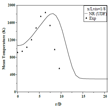
The radial profiles of mean mixture fraction are shown to gether with the experimental data in figures 2 and 3, for the two axial position (x/Lvis = 1/8and3/4). At x/Lvis = 1/8, the numerical results under predict the experimental data at the center axis and slightly over predict them in the radial distance regions near the center axis (5 ≤ r/Rj≤ 10). This under prediction begins to decrease in the regions away from the nozzle exit (at x/Lvis = 3/4). The experimental data are well predicted. Figure 4 shows the axial evolution of mean temperature. This evolution presents the same behavior as that of experience. The maximum value, which is slightly over predicted in amplitude, is in axial position the same. This axial position (x/Lvis ≈ 0.66) corresponds to the stoichiometric value of the mixture fraction Zst ≈ 0.028.
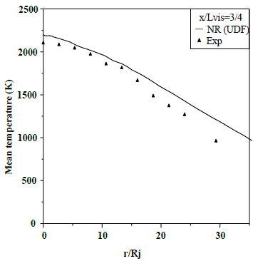
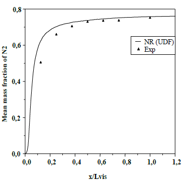
The radial profiles of mean temperature are shown in figures 5 and 6. the numerical results tend to over predict the experimental data in the region close to the nozzle exit (at x/Lvis=1/8), however, they predicts best the experimental results in the radial distance regions very close to the center axis (r/Rj≤ 4). The temperature peak is in good agreement with experimental data and its radial position is relativelyclose to this of experiment. In the far region (at x/Lvis=3/4), numerical results are in good agreement with experimental data. The numerical results predictions of mean profiles of mass fraction of hydrogen, water, oxygen and nitrogen are shown in Figs. 7, 8, 9 and 10, respectively. The numerical results of are in good agreement with experimental data. The mean mass fraction of H2 presents the same behavior as that of mixture fraction. In the region close to the nozzle exit (x/Lvis≤ 0.2), numerical results under predict the experimental values of mean mass fraction of O2.
The difference between numerical simulation and experimental results may be due to the upstream conditions affecting very much the initial zone of the jet and/or to the effect of preferential diffusion[21], [22] that characterize the hydrogen turbulent flames. The non-equilibrium chemistry [21] and/or model of turbulence used may also play an important role in this region.
Figure 3. Radial profile of mean mixture fraction at x/Lvis= 3/4
Figure 4. Axial profile of mean temperature
Figure 5. Axial profile of mean temperature at x/Lvis= 1/8
Figure 6. Radial mean temperature profile at x/Lvis= 3/4
Figure 7. Mean mass fraction of H2
Figure 8. Mean mass fraction of H2O
Figure 9. Mean mass fraction of O2
Figure 10. Mean mass fraction of N2
A consistent hybrid RANS–TPDF method has been proposed for the simulation of hydrogen turbulent jet diffusion flame. The flow field has been solved on the basis of the RSM model. A modeled scalar PDF equation has been solved by a Lagrangian Monte Carlo method developed by Pope [6].This provides a detailed modeling of the turbulence chemistry interaction. The molecular mixing term is modeled by EMST model. An algebraic model of the time scale ration CΦ, obtained from DNS calculation [4] was used and implemented, in FLUENT 13.0 code, via a so-called User Defined Function (UDF).
On the basis of obtained result, we can draw the following conclusions:
|
Roman symbols |
|
|
|
k |
Turbulent kinetic energy |
|
|
P |
Instantaneous Pressure |
|
|
R |
Perfect gas constant |
|
|
r |
Radial distance |
|
|
Ret |
Turbulent Reynolds number |
|
|
Rt |
Time-scale ratio or mixing-model constant |
|
|
Sct |
Turbulent Schmidt number |
|
|
t |
Time |
|
|
T |
Instantaneous temperature |
|
|
$u_{i}$ |
Velocity in direction i |
|
|
$u_{i}^{\prime \prime}$ |
Favre fluctuations of velocity in direction i |
|
|
Yα |
Species mass fraction of species α |
|
|
Wα |
Atomic weight of species α |
|
|
Greek symbols |
|
|
|
$\varepsilon$ |
Dissipation rate of turbulent energy |
|
|
$\mathbb{\Phi}$ |
Scalar variable (species mass fractions or enthalpy) |
|
|
$\mu_{e f f}$ |
The effective viscosity (molecular and turbulent viscosity) |
|
|
ν |
Kinematic viscosity |
|
|
$\rho$ |
Density |
|
|
$\delta_{i j}$ |
Kronecker delta |
|
|
Conventions |
||
|
— |
Reynolds average (Conventional average) |
|
|
~ |
weighted averaging) |
|
|
$( .)_{i j}$ |
Tensorial notation with summation on the repeated indices |
|
|
$( .)_{t}$ |
Turbulent |
|
|
Abbreviation |
|
|
|
CFD |
Computetionel Fluid Dynamics |
|
|
DNS |
Direct Numerical Simulation |
|
|
EMST |
Euclidean Minimum Spanning Tree |
|
|
IEM |
Interaction by Exchange with the Mean. |
|
|
JCMDF |
Joint Composition Mass Density Function |
|
|
JPDF |
Joint Probability Density Function |
|
|
LES |
Large-Eddy Simulation. |
|
|
MDF |
Mass Density Function. |
|
|
NR |
Numerical results |
|
|
|
Probability density function. |
|
|
RANS |
Reynolds-Averaged Navier-Stokes |
|
|
RSM |
Reynolds Stress Model. |
|
|
UDF |
User Defined Function |
|
[1] Dopazo, C. and O’Brien, E. E., “Approach to autoignition of a turbulent mixture,” Acta Astronaut, 1, 1974, pp. 1239. DOI: 10.1016/0094-5765(74)90050-2.
[2] Subramaniam, S. and Pope, S. B., “A mixing model for turbulent reactive flows based on Euclidean minimum spanning trees,” Combust. Flame, 1998, pp.115-487.
[3] Senouci, M., Bounif, A., Abidat, M., Belkaid, N. M., Mansour and C., Gokalp, I., “Transported-PDF (IEM, EMST) micromixing models in a hydrogen-air non premixed turbulent flame,” Acta Mechanica, vol. 224, no. 27, 2013. DOI : 10.1007/s00707-013-0911-5.
[4] Overholt, M. R. and Pope, S. B., “Direct numerical simulation of a passive scalar with imposed mean gradient in isotropic turbulence,” Phys. Fluids, vol. 8, pp. 3128-3148, 1996. DOI: 10.1063/1.869099.
[5] Barlow, R. S., Sandia H2/He Flame, http://www.ca.sandia.gov/TNF, 2003.
[6] Pope, S. B., “PDF methods for turbulent reactive flows,” Progress in Energy Combustion Science, vol. 11, 1985, pp. 119–192.
[7] Pope, S. B., “Lagrangian PDF methods for turbulent flows,” Annual Review of Fluid Mechanics, vol. 26, pp. 23- 63, 1994.
[8] Cao, R. R., Pope, S. B. and Masri, A. R., “Turbulent lifted flames in a vitiated coflow investigated using joint PDF calculations,” Combustion and Flame, vol. 142, pp. 438–453, 2005.
[9] Xu, J. and Pope, S.B., “Combust,” Flame, vol. 123, pp. 281–307, 2000.
[10] Lindstedt, R. P., Louloudi, S. A. and Vaos, E. M., Proc. Com- bust. Inst., vol. 28, pp. 149–156, 2000.
[11] Dopazo, C., “Probability density function approach for a turbulent axisymmetric heated jet,” Centreline evolution.Phys. Fluids, vol. 18, no. 4, pp.397-404, 1975.
[12] Naud, B., Jiménez, C. and Roekaerts, D., “A consistent hybrid PDF method, implementation details and application to the simulation of a bluff-body stabilised flame,” Progress in Computational Fluid Dynamics, vol. 6, pp. 146-157, 2006. DOI: 10.1504/PCFD.2006.009492.
[13] Heinz, S. and Roekaerts, D., “Reynolds number effects on mixing and reaction in a turbulent pipe flow,” Chem. Engrg. Sci., vol. 56, pp. 3197–3210, 2001.
[14] Pope, S. B., Turbulent Flows, Cambridge University Press, pp. 200, 2000. DOI: 10.1017/CBO9780511840531.
[15] Barlow, R. S., Carter, C. D., “Raman/Rayleigh/Lif measurements of nitric oxide formation in turbulent hydrogen jet flames,” Combust. Flame, vol. 97, pp. 261–280, 1994. DOI: 10.1016/0010-2180(94)90020-5.
[16] Luppes, R., “The numerical simulation of turbulent jets and diffusion flames,” Technische Universiteit Eindhoven Netherlands, pp. 51-55, 2000.
[17] Zijlema, M. “Computational modelling of turbulent flow in general domains,” PhD thesis, Delft University of Technology, The Netherlands, 1996.
[18] Fairweather, M. and Woolley, R. M., “First order conditional moment closure modeling of turbulent nonpremixed hydrogenflames,” Combust. Flame, vol. 133, pp. 393–405, 2003.
[19] Obieglo, A., Gass, J. and Poulikakos, D., “Comparative study of modeling hydrogen nonpremixed turbulent flame,” Combust. Flame, vol. 122, pp. 176–194, 2000.
[20] Zijlema, M., “Computational modelling of turbulent flow in general domains,” PhD thesis, Delft University of Technology, The Netherlands.1996.
[21] Meier, W., Vyrodov, A. O., Bergmann, V. and Stricker, W., “Simultaneous Raman/LIF measurements of major species and NO in turbulent H2/air diffusion flames,” Appl. Phys. B, pp. 63 -79- 90, 1996.
[22] Sanders, H., “Non equilibrium and differential diffusion effects in turbulent hydrogen diffusion flames,” J. Thermophys. Heat Transf., vol. 11, pp. 384–390, 1997.
[23] A. Tariq, A., Azab and Essa, A., “Effect of rectangular perforation aspect ratio on fin performance,” International Journal of Heat and Technology, vol.28, no.1, pp. 53-60, 2010.
[24] S. Suneeeta, P. Gajanan and S. Narayan, “Experimental analysis of natural convection heat transfer from horizontal rectangular notched fin arrays,” International Journal of Heat and Technology, vol.27, no. 2, pp. 9-14, 2009.