OPEN ACCESS
Experimental and Theoretical investigation is presented to simulate the heat transfer in flat-plate single pass solar air collector working in forced convection. The complexity of the mathematical models of these phenomena has led researchers to conduct studies related to this field based on several simplifying assumptions, such as, the convective heat transfer coefficient is considered as constant. In this research work, initially, an experimental study is performed using thermocouples to measure temperature distributions on solar air heater components. The different measured temperatures of the absorber plate, air flow and bottom plate are used to determine the local convective heat transfer coefficients. Secondly, the problem is treated numerically by a developed FORTRAN code to calculate, for different solar radiation intensity, the temperature variations in each solar air panel components. Satisfactory qualitative and quantitative agreement is obtained between the numerical and experimental results.
Local convective heat transfer coefficients, Solar air collector, Efficiency factor, Convection.
Energy in various forms has played an increasingly important role in worldwide economic progress and industrialization. Due to several economic and environmental benefits, solar energy transformed into heat has found many applications in the field of heating, drying, cold production, etc. [1-7].
Solar thermal collectors, which allow the production of thermal energy, convert solar radiations into heat energy extracted by air flow through the collector. The calculation of their performance, based on the understanding of flow and heat transfer mechanisms in their different parts, is usually carried out with uniform average heat transfer coefficients. However, in practical operation, the heat transfer over absorbers is related to the air flow structure which varies from the bottom to the top of the panels [8]. Thus, in order to conduct an accurate analysis on the thermal performance of the tested flat-plate single pass solar air collector, the local convective heat transfer coefficients must be determined. In this work, we estimate these local convective coefficients.
Many researchers [9-11] have investigated theoretically the different collector designs by applying the heat balance equations in order to compute the temperature distribution in each of their components. In the calculations, the heat transfer coefficients, which are assumed constant over the flow channels, were determined from the correlation developed by Kays [12]. Ong [9] used this method to predict the heat transfer characteristics of four types of solar air heaters. The effects of pertinent parameters on the system efficiencies were discussed. Among his results, he found that satisfactory results could be achieved for a collector length equal to 1 m. Using the same theoretical method. Bahrehmand and Amri [13] studied single and two-glass cover solar air heaters with natural convection flow. Their goal was to show the effect of longitudinal fins, as well as the depth and length variations of the channel on energy and exergy performances of the collectors. They noticed that the devices with two-glass are more efficient than a single glass collectors. Sopian et al. [10] developed the theoretical and experimental models in the transient regime in order to analyze the thermal performance of the double-pass solar collector with porous media. They obtained a close agreement of the thermal efficiency between the theoretical and experimental approaches.
Several experimental articles have been presented in the litterature on solar air heaters. Ong [13] experimentally analyzed the performance of three types of single pass solar air heaters. One of them was studied with and without bottom insulation. The author validated his theoretical model [9 ] by comparing the predicted results with those measured experimentally. Mokhtari and Semmar [14] conducted an experimental study on the thermal performance of three types of single solar air heaters. The geometries of these three configurations differ from one to another by the position and the shape of the flow channel. Basing on the measured outlet temperature, it was noticed that the collector having a diagonally positioned absorber has a better efficiency than the two other configurations. Koyuncy [15] experimentally investigated the performance of different collector designs in order de determine the most efficient and the easiest to manufacture and whith high efficiency for low temperature crop drying systems.
Several experimental and numerical studies have been considered in order to estimate the local convective heat transfer coefficients. For example, Saboya and Sparrow [16] and Yoo et al. [17] used a naphthalene sublimation technique to measure the local coefficients in the heat exchangers. The inverse problems of heat conduction are among the most widely used to determine these coefficients. Huang et al. [18] and Benmachiche et al. [19] applied the conjugate gradient method, which is based on an inverse algorithm scheme, to estimate the local heat transfer coefficients over finned-tube heat exchangers. Ay et al. [20] presented a local study of the heat transfer coefficient over the plate fin inside heat exchangers. The computations were based on the finite difference method and on the temperature distribution obtained by the infrared thermography technique.
Other works have been carried out to determine the convective heat transfer coefficients in solar air heaters. Moummi et al. [21] gave an approximate approach to calculate these coefficients in flat plate solar air collectors provided with rectangular plate fins placed perpendicular to the flow. They compared their results with those obtained for a solar collector without fins. Hatami and Bahadorinejad[ 22 ] conducted an experimental study for the determination of the average natural convection heat transfer coefficients in a vertical flat plate solar collector with single and double glass covers. Their study covered six operational modes for two cases (vertical channels and enclosures). They proposed a Nusselt number correlation for each studied case. Gao et al. [23] carried out a numerical study of natural convection heat transfer inside the channel between the flat-plate cover and the sine-wave absorber in a cross corrugated solar air heater. The Navier Stokes and energy equations were solved using the finite volumes method to estimate the average heat transfer coefficient. The authors investigated the effects of system parameters, such as the wavelike absorber characteristics, on the estimated coefficient.
In this work, we have determined experimentally the local convective heat transfer coefficients from the measured temperatures of the absorber plate, the air flow and the bottom plate. Then, we have used these coefficients to predict the temperature distribution in the solar air collector via a mathematical model obtained from the energy balance in the system. A comparison between the measured and predicted temperature distributions is conducted through different solar radiation intensity.
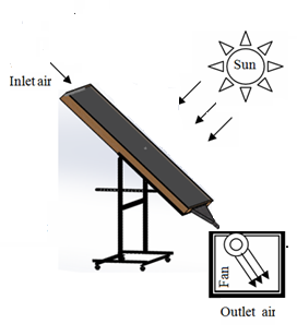
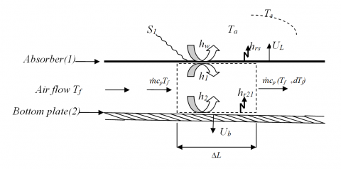
The thermal analysis for predicting the performance of different types of solar air collectors has been presented by many investigators [9, 10]. The mathematical models of these devices are based on energy balance over each of their elements. The mean difference between them lies in the estimated heat transfer coefficients and in the numerical solving procedures. In order to simplify the problem, numerous investigations have been carried out by considering that the plates are maintained at the main temperatures [22]. However, in solar air heaters, these temperatures vary along their length. Therefore, for accurate thermal simulations, we use a discrete approach which consists of dividing the collector into several differential elements in the air flow direction. The solar energy system modeled in the present work is shown in Figs. (1, 2), energy balance is then applied in each element considered as a control volume. In each control volume, the air temperature is assumed to vary linearly which is valid for short collectors (less than 10 m) [9].
The mean air temperature is then:
$T_{f}=\left(T_{f, i}+T_{f, o}\right) / 2$
where $T_{f, i}$ and $T_{f, o}$ are the inlet and the outlet temperatures, respectively.
Figure 1. Diagrams of the studied model.
Figure 2. Schematic representation of heat transfer in the different collector components.
2.1 Simplifying assumptions
The energy equations for the different elements of the solar air collectors in conservation form are formulated making the following assumptions:
•The system operates under steady state conditions;
•Air, absorber and bottom plate temperatures change only in the direction of the air flow;
•Air temperature is assumed uniform through the cross section;
•Heat conduction is considered negligible;
•Outside convective heat transfer coefficient is constant along the length of solar air heater.
2.2 Energy balance equations
The following energy balance equations are written for various collector components in each control volume:
For the absorber plate:
$S_{1}+h_{r 21}\left(T_{2}-T_{1}\right)+h_{1}\left(T_{f}-T_{1}\right)=U_{L}\left(T_{1}-T_{a}\right)$(1)
For the air flow:
$h_{2}\left(T_{2}-T_{f}\right)=h_{1}\left(T_{f}-T_{1}\right)+Q$(2)
For the bottom plate:
$h_{2}\left(T_{f}-T_{2}\right)+h_{r 21}\left(T_{2}-T_{1}\right)=U_{b}\left(T_{2}-T_{a}\right)$(3)
The useful heat transferred to air can be written in terms of the mean fluid and inlet temperatures as follows:
$Q=\Gamma\left(T_{f}-T_{f, i-1}\right)$(4)
$\Gamma=\dot{m} C p /(W \Delta x)$(5)
2.3 Estimation of heat transfer coefficients
In order to identify the external convective heat transfer coefficient due to wind outside the collector, the correlation proposed by McAdams [24] is used :
$h_{w}=5.7+3.8 V$(6)
The convective heat transfer coefficients between air flow and glass, and between the absorber plate and the bottom plate for turbulent (Re≥ 2300) forced convection flow can be determined using the follwing correlation [12]:
$N u=\frac{h D_{h}}{K}=0.0158 \mathrm{Re}^{0.8}$(7)
where
$D_{h}=\frac{4 A}{P}$(8)
The solar radiation heat flux absorbed by the absorber is:
$S_{1}=\alpha . G$(9)
The radiative heat transfer coefficient between the glass and the sky is obtaind from the formula:
$h_{r s}=\frac{\sigma \varepsilon_{1}\left(T_{1}+T_{s}\right)\left(T_{1}^{2}+T_{s}^{2}\right)\left(T_{1}-T_{s}\right)}{\left(T_{1}-T_{a}\right)}$(10)
The temperature of the sky is [25]:
$T_{s}=0.0552 \mathrm{Ta}^{1,5}$(11)
The radiative heat transfer coefficient between the absorber and the lower plate is given by:
$h_{r 21}=\frac{\sigma\left(T_{1}^{2}+T_{2}^{2}\right)(T 1+T 2)}{\frac{1}{\varepsilon_{1}}+\frac{1}{\varepsilon_{2}}-1}$(12)
The coefficient of heat losses toward the rear of the solar air collector is defined as:
$U_{b}=\frac{1}{i=\Sigma_{1}^{n} \frac{X_{b i}}{k_{b i}}+\frac{1}{h_{w}}}$(13)
The coefficient of heat losses to the front of the solar air collector is defined as:
$U_{L}=h_{w}+h_{r s}$(14)
2.4 Solution method
In each control volume, the difference method is applied to approximate the air temperature gradient as follows:
$\frac{d T_{f}}{d x} \approx \frac{T_{f, i}-T_{f, i-1}}{\Delta x}$
Substituting this equation into Eq. 4. The above Eqs. (1-14) can be written in a 3x3 matrix form [A] [T] = [B]. Where:
$[A]=\left[\begin{array}{ccc}{\left(h_{1}+h_{r 21}+U_{l}\right)} & {-h_{1}} & {-h_{r 21}} \\ {h_{1}} & {-\left(h_{1}+h_{2}+\Gamma\right)} & {h_{2}} \\ {-h_{r 21}} & {-h_{2}} & {\left(h_{2}+h_{r 21}+U_{b}\right)}\end{array}\right]$
$[T]=\left[\begin{array}{l}{T_{1}} \\ {T_{f}} \\ {T_{2}}\end{array}\right]$ And $[B]=\left[\begin{array}{c}{U_{l} T_{a}+S_{1}} \\ {-\Gamma T_{f, i-1}} \\ {U_{b} T_{a}}\end{array}\right]$
Gauss elimination algorithm is used to calculate the unknown temperatures T1, T2, Tf.
The elements of the matrix [A] contain radiative heat transfer coefficients which depend on the unknown temperatures; an iterative process based on substitution technique was then carried out in each control volume.
3.1 Description of the considered solar air heater
An experimental set-up was designed and tested in the University of Biskra. Biskra is a city located in the East of Algeria with latitude of 34°48' N, longitude of 5°44'E and altitude of 85 m. The studied solar energy system is a flat-plate solar air heater with a single air flows between the absorber and the bottom plate placed on the insulator. The collector is placed on a stand facing south. To measure temperatures, type K thermocouples were connected at appropriate locations to a digital temperature indicator with 0.1°C least count. The layout of the studied solar air collector which is shown in Fig. 3 is designed with the following parameters:
•Solar collecting area was 2 m length× 1 m width;
•Installation angle of the collector was 34°48' from horizontal;
•Height of the stagnant air layer was d= 0.04 m;
•Black paint absorber with a thickness of 1 mm and absorption coefficient of α= 0.95 was made of galvanized steel sheet;
•Expanded polystyrene board with thermal conductivity of 0.037W/m. K was used for insulating the collector rear;
•A CMP 3 Pyranometer was used to measure solar irradiance; a digital thermometer Model Number: DM6802B was also used;
•6 positions of thermocouples connected to absorber plate;
•6 positions of thermocouples connected to bottom plate;
•6 positions of thermocouples connected with the air flow.
Figure 3. Photgraph of experimental set-up
3.2 Collector thermal efficiency
The efficiency of a solar air collector is defined as the ratio of the amount of useful heat collected to the total amount of solar radiation striking the collector surface:
$\eta=\frac{Q_{u}}{G \cdot A}$(15)
The average useful heat collected for an air solar collector can be expressed as:
$Q_{u}=\dot{m} C_{p}\left(T_{o u t}-T_{i n}\right)$
So, collector thermal efficiency becomes:
$\eta=\dot{m} C_{p} \frac{\left(T_{o u t}-T_{i n}\right)}{G . A}$(16)
3.3 Calculation of the local convective heat transfer coefficient
In the present article, the coefficients for upper and lower surfaces of channel were assumed equal: h1= h2.
Local convective heat transfer coefficients between the fluid and the absorber plate are described by using energy balance equations and they are evaluated at a given position by this relationship:
$h(x)=\frac{U_{L}(x)\left(T_{1}(x)-T_{a}\right)-h_{r 21}(x)\left(T_{2}(x)-T_{1}(x)\right)-s_{1}}{T_{f}(x)-T_{1}(x)}$(17)
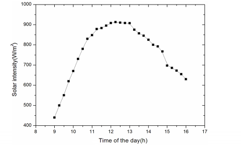
Thermal efficiency $\eta$ is usualy used to evaluate the performance of solar air heaters. Figs (4,5) show the variation of the experimental thermal paramater and solar intensity,respectively, as a function of time for a value of air mass flow rate equal to 0.1324 Kg/s which corresponds to Re=38381. It can be noted from these figures that the thermal efficiency increases with the solar intensity. It is also apparent that the highest solar intensity produces the highest thermal efficiency. The maximum value of $\eta$ is 40% for solar intensity G=845W/m2 measured at 13:30 and its minimum value is 22.5% for G=440W/m2 measured at the time of the air heater started to use.
Fig. 6 illustrates the variation of the measured inlet and outlet temperatures with time. For a tested Reynolds number (Re= 38381.1), the outlet and inlet temperatures of the air flow increase from morning to a peak values at noon and then decrease in the afternoon. As expected, it can be also seen from this figure that the variations of the outlet temperature are significant.
Our proposed model implemented for the calculation of local convective heat coefficient between air flow and the absorber plate (eq.17) is validated using two procedures:
i) First, by comparison with the results obtained from the Nusselt number correlation [10], see Figs. (8, 10, 12 and14).
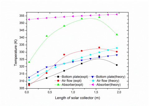
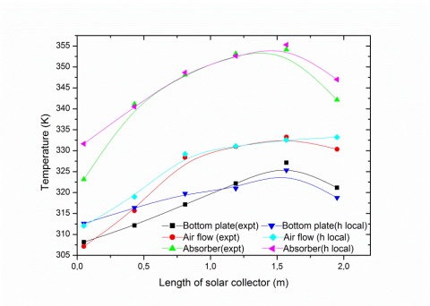
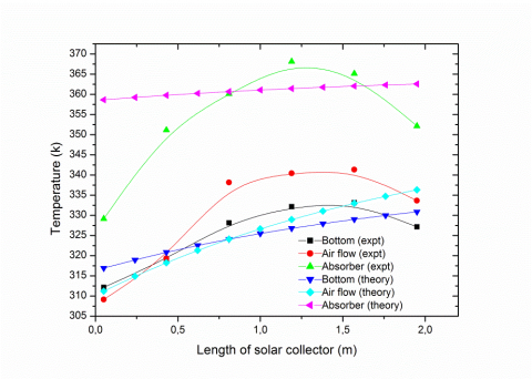
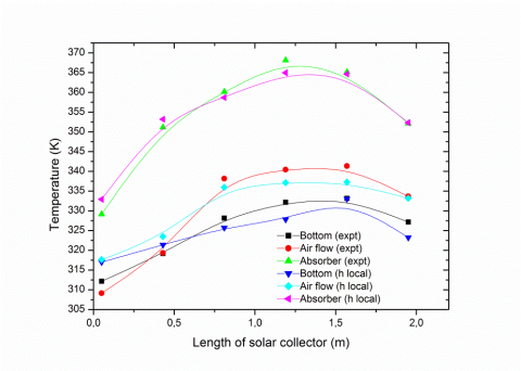
ii) Secondly, by comparing the calculated temperatures using our model with their experimental values, see Figs (9, 11, 13 and15).
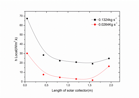
The local heat transfer coefficients h have been estimated and represented in Fig.7 for two values of air mass flow rate $\dot{m}$ . This figure gives clear indications of the dependence of these local coefficients on air mass flow. In fact, they increase with the Reynolds number. It can be observed from this figure that their maxima are always located at the front part of the collector regardless of the Reynolds number value. This is in full accordance with the concept of the boundary layer formation.
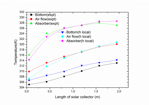
For a better appreciation of the proposed estimation of h, we compare the experimental and theoretical values of the temperatures in Figs. (8-15). That is the measured temperatures, the temperatures obtained from the correlation given by Eq. (7) and the temperatures computed using Eq. (17). It can be noticed that, as expected, for the used values of the Reynolds numbers and of the solar intensity, the temperatures over each component of the solar collector increase along the collector in the direction of air flow. The comparison between the results of the two approaches (Figs. (9, 11, 13 and 15)), reveals that the local convective heat transfer coefficients estimated from Eq. (17) offers very good agreement with experimental results.
In order to examine the use of the predicted local heat transfer coefficient in the calculation of the temperatures we proceed as follows:
First, we estimated the values of the coefficients h using the experimental temperatures for a given value of the solar radiation intensity (G =680W/m2). Then, we injected these estimated values of h in our FORTRAN code in order to compute numerically the temperatures for different new values of the radiation intensity and for two Reynolds numbers (Re=3839.1 and Re=38381.6): i) For Re=3839.1, Figs. 9 and 11 summarize the results for two values of G (Figs. 9 for G=750W/m2 and Fig. 11for G=850W/m2); ii) for Re=38381.6, Figs. 13 and 15 show the results for two other values of G (Figs. 13 for G=700 W/m2 and Fig. 15 for G=900W/m2). It is clear from these figures that there is a good agreement between the calculated and experimental values of the temperature along air flow direction. This cofirms the fiability of our predected local transfer coefficents and the consolidates the validity of our numerical model
It is seen from Figs. (8-15) that, for all studied cases, air and plates temperatures increase along the panel up to about 1.5 m length, beyond this zones these temperatures remain relatively constant. We noticed as well that the experimental temperatures decrease at the end of the panel. This can be due to the geometrical shape of the collector output which disturbs the flow and creates flow recirculation in this area. This effect contributes to lower the temperature within the downstream area of the collector
Figure 4. Solar intensity versus time of day,with Re=38381.6 (26/06/2014)
Figure 5. Variation of efficiency versus time of day,with Re=38381.6 (26/06/2014)
Figure 6. Variation of the outlet and inlet temperatures deponing on the time at Re=38381.6,(26/06/2014)
Figure 7. Variation of the local convective heat transfer coefficient according to the solar air collector length for G=680W/m2
Figure 8. Numerical and experimental temperatures variations along solar collector, with Re=3839.1, G=750W/m2
Figure 9. Numerical (using local heat transfer coefficient) and experimental temperatures variations along solar collector, with Re=3839.1, G=750W/m2
Figure 10. Numerical and experimental temperatures variations along solar collector, with Re=3839.1, G=750W/m2
Figure 11. Numerical (using local heat transfer coefficient) and experimental temperatures variations along solar collector, with Re=3839.1, G=850W/m2
Figure 12. Numerical and experimental temperatures variations along solar collector, with Re=38381.6, G=700W/m2
Figure 13. Numerical (using local heat transfer coefficient) and experimental temperatures variations along solar collector, with Re=38381.6, G=700W/m2
Figure 14. Numerical and experimental temperatures variations along solar collector, with Re=38381.6, G=900W/m2
Figure 15. Numerical (using local heat transfer coefficient) and experimental temperatures variations along solar collector, with Re=38381.6, G=900W/m2.
In this work, we have proposed a theoretical model which consists of dividing the collector into several differential elements along the collector. Thermal balance is then applied over each element in conjunction with the measured temperatures in order to predict the local heat transfer coefficients in the air flow channel. From the FORTRAN numerical code that we have developed and using these coefficients, we have computed the temperatures profiles of the absorber plate, air flow and bottom plate. The numerical calculation of temperature distributions is done for several values of the solar radiation intensity. The results of the proposed approach agree closely with values measured experimentally.
|
Symbols |
|
|
|
$T_{1}$ |
absorber plate temperature, (K) |
|
|
$T_{2}$ |
Bottom plate temperature, (K) |
|
|
$T_{f}$ |
Air flow temperature, (K) |
|
|
$T_{a}$ |
Ambient temperature, (K) |
|
|
$T_{S}$ |
Sky temperature, (K) |
|
|
$G$ |
Incident solar radiation, (W/m2) |
|
|
$h_{1}$ |
Convective heat transfer coefficient between the absorber and the air flow, (W/m2 K) |
|
|
$h_{2}$ |
Convective heat transfer coefficient between the bottom plate and the air flow, (W/m2 K) |
|
|
$h_{r 21}$ |
radiation heat transfer coefficients,(W/m2 K) |
|
|
$h_{r s}$ |
radiation heat transfer coefficient, (W/m2 K) |
|
|
$h_{w}$ |
wind convection heat transfer coefficient, (W/m2 K) |
|
|
Cp |
Isobaric specific heat of air, (J/kg K) |
|
|
$K_{f}$ |
thermal conductivity of air flow, (W/m K) |
|
|
$k_{b i}$ |
thermal conductivity of insulation, (W/m K) |
|
|
$U_{L}$ |
Top loss heat coefficient, (W/m2 K) |
|
|
$U_{b}$ |
Bottom heat loss coefficient, (W/m2 K) |
|
|
$\dot{m}$ |
mass flow rate, (Kg/s) |
|
|
$W$ |
Wind velocity, (m/s) |
|
|
$N u$ |
Nusselt number |
|
|
$R e$ |
Reynolds number |
|
|
$W$ |
width of collector, (m) |
|
|
$L$ |
length of collector, (m) |
|
|
$X_{b i}$ |
insulation thickness, (m) |
|
|
$d$ |
spacing between absorber and bottom surfaces, (m) |
|
|
$D_{h}$ |
equivalent diameter, (m) |
|
|
$A$ |
cross section of flow area, (m2) |
|
|
$P$ |
wetted perimeter, (m) |
|
|
$Q$ |
heat transferred to air streams |
|
|
Greek symbols |
||
|
$\varepsilon_{1}$ |
emissivity of black absorber upper surface |
|
|
$\varepsilon_{2}$ |
emissivity of unpainted absorber lower surface |
|
|
$\alpha$ |
Absorptivity of absorber plate |
|
|
$\rho$ |
density of air, (Kg/m3) |
|
|
$\Sigma$ |
Stefan–Boltzmann constant |
|
|
$\mu$ |
dynamic viscosity of air, (kg m-1 s-1) |
|
[1] J. Duffe and W. Beckman, Solar Engineering of Thermal Processes, New York: Wiley, 1991.
[2] T. Koyuncu, “Performance of various design of solar air heaters for crop drying applications,” Renewable Energy, vol. 31 no. 7, pp. 1073-1088, 2006. DOI: 10.1016/j.renene.2005.05.017.
[3] S. Chemkhi, F. Zagrouba and A. Bellagi, “Drying of agricultural crops by solar energy,” Desalination, vol. 168, pp. 101-109, 2004. DOI: 10.1016/j.desal.2004.06.174.
[4] F. K. Forson, M. A. Nazha, F. O. Akuffo and H. Rajakaruna, “Design of mixed-mode natural convection solar crop dryers: application of principles and rules of thumb,” Renewable Energy, vol. 32, pp. 2306–2319, 2007. DOI: 10.1016/j.renene.2006.12.003.
[5] D. R. Pangavhane, R. L. Sawhney and P. N. Sarsavadia, “Design, development and performance testing of a new natural convection solar dryer,” Energy, vol. 27, pp. 579–590, 2002. DOI: 10.1016/S0360-5442(02)00005-1.
[6] M. Coppi, A. Quintino and F. Salata, “Fluid dynamic feasibility study of solar chimney in residentail buildings,” International Journal of Heat and Technology, vol. 29, pp. 1-6, 2011.
[7] Bernardo Buonomo, Orazio Manca, Sergio Nardini and Paolo Romano, “Thermal and fluid dynamic analysis of solar chimney building systems,” International Journal of Heat and Technology, vol. 31, pp. 19-126, 2013.
[8] R. Ben Slama, “The air solar collectors: Comparative study, introduction of baffles to favor the heat transfer,” Solar Energy, vol. 81, pp. 139-149, 2007. DOI: 10.1016/j.solener.2006.05.002.
[9] K. Ong, “Thermal performance of solar air heaters: mathematical model and solution procedure,” Solar Energy, vol. 55, pp. 93–109, 1995a. DOI: 10.1016/0038-092X(95)00021-I.
[10] K. Sopian, M. A. Alghoul, Ebrahim M. Alfegi, M. Y. Sulaiman and E. A. Musa, “Evaluation of thermal efficiency of double-pass solar collector with porous–nonporous media,” Renewable Energy, vol. 34, pp. 640-645, 2009. DOI: 10.1016/j.renene.2008.05.027.
[11] D. Bahrehmand and M. Ameri, “Energy and exergy analysis of different solar air collector systems withnatural convection,” Renewable Energy, vol. 74, pp. 357-368, 2015. DOI: 10.1016/j.renene.2014.08.028.
[12] Kays W. M., Convective Heat and Mass Transfer. New York: McGraw-Hill, 1980.
[13] K. Ong, “Thermal performance of solar air heaters: experimental correlation,” Solar Energy, vol. 55, pp. 209–220, 1995b. DOI: 10.1016/0038-092X(95)00027O.
[14] F. Mokhtari and D. Semmar, “L’influence de la configuration de l’absorbeur sur les performances thermiques d’un capteur solaire à air,” Revue des Energies Renouvelables: Days Thermal, pp. 159-162, 2001.
[15] T. Koyuncu, “Performance of various designs of solar air heaters for crop drying applications,” Renewable Energy, vol. 31, pp. 1073-1088, 2006. DOI: 10.1016/j.renene.2005.05.017.
[16] F. E. M. Saboya and E. M. Sparrow, “Experiments on a three row fin and tube heat exchanger,” J. Heat Transfer, vol. 19, pp. 26–34, 1976.
[17] S. Yoo, H. Kwon and J. Kim, “A study on heat transfer characteristics for staggered tube banks in cross-flow,” J. of Mechanical Science and Technology, vol. 21, pp. 505-512, 2007. DOI: 10.1007/BF02916312.
[18] C. H. Huang, I. C. Yuan and H. Ay, “A three-dimensional inverse problem in imaging the local heat transfer coefficients for plate finned-tube heat exchangers,” Int J Heat and Mass Transfer, vol. 46, pp. 3629-3638, 2003. DOI: 10.1016/S0017-9310(03)00157-1.
[19] A. H. Benmachiche, C. Bougriou and S. Abboudi, “Inverse determination of the heat transfer characteristics on a circular plane fin in a finned-tube bundle,” Heat and Mass Transfer, vol. 46, pp. 1367-1377, 2010. DOI: 10.1007/s00231-010-0664-9.
[20] H. Ay, J. Y. Jang and J. N. Yeh, “Local heat transfer measurements of plate finned-tube heat exchangers by infrared thermography,” Heat and Mass Transfer, vol.45, pp. 4069-4078, 2002.
[21] N. Moummi, S. Youcef-Ali, A. Moummi and J. Y. Desmons, “Energy analysis of a solar air collector with rows of fins,” Renewable Energy, vol. 29, pp. 2053–2064, 2004. DOI: 10.1016/j.renene.2003.11.006.
[22] N. Hatami and M. Bahadorinejad, “Experimental determination of natural convection heat transfer coefficient in a vertical flat-plate solar air heater,” Solar Energy, vol. 82, pp. 903-910, 2008. DOI: 10.1016/j.solener.2008.03.008.
[23] W. Gao, W. Lin and E. Lu, “Numerical study on natural convection inside the channel between the flat-plate cover and sine-wave absorber of a cross-corrugated solar air heater,” Energy Conversion & Management, vol. 41, pp. 145-151, 2000. DOI: 10.1016/S0196-8904(99)00098-9.
[24] W. H. McAdams, Heat Transmission, third ed. New York: McGraw-Hill, 1954.
[25] W. C. Swinbank, “Long-wave radiation from clear skies,” Q. J. R. Meteorol. vol. 89, 1963.