OPEN ACCESS
This paper presents a numerical study of natural convection cooling of water-Al2O3 nanofluid by two heat sinks vertically attached to the horizontal walls of a cavity subjected to a magnetic field. The left wall is hot, the right and the horizontal walls are insulated. Lattice Boltzmann method (LBM) is applied to solve the coupled equations of flow and temperature fields. This study has been carried out for the pertinent parameters in the following ranges: Rayleigh number of the base fluid, Ra = 103 to 105, Hartmann number varied from Ha = 0 to 60 and the solid volume fraction of nanoparticles between $\Phi$= 0 and 6%. In order to investigate the effect of heat sinks location, three different configurations of heat sinks are considered. Results show that the heat sinks positions greatly influence the heat transfer rate depending on the Hartmann number, Rayleigh number and solid volume fraction of nanoparticles.
Heat sink, Lattice Boltzmann Method, Magnetic field, Nanofluid, Natural convection.
Natural convection in square enclosures has many engineering applications such as cooling systems of electronic components, solar collectors, thermal storage systems and nuclear reactor systems. Therefore, it is important to understand the thermal behavior of such systems when the natural convection is the dominant mode of heat transfer. The low thermal conductivity of conventional heat transfer fluids, commonly water, has restricted designers. Adding some solid nanoparticles with high thermal conductivity to the fluid is one of the ways to overcome this problem. The resulting fluid is a suspension of the solid nanoparticle in the base fluid which is called “nanofluid”. The thermal conductivities of nanofluids are believed to be greater than the base fluid due to the high thermal conductivity of the nanoparticles. The Lattice Boltzmann Method (LBM) is an applicable method for simulating fluid flow and heat transfer [1–3]. This method was also applied to simulate Magnetohydrodynamic (MHD) and, recently, nanofluid successfully. Mejri et al. [4-8] studied the laminar natural convection and entropy generation in a square enclosure, with sinusoidal temperature distribution, filled with a water-Al2O3 nanofluid and is subjected to a magnetic field. Mahmoudi et al. [9-11] studied the effect of magnetic field and its direction on water-Al2O3 nanofluid filled cavity with a linear boundary condition, the results show that the magnetic field direction controls the flow and heat transfer rates in the cavity. Mahmoudi et al. [12-13] studied MHD natural convection in a square cavity filled with nanofluid. The results show that adding nanoparticle increases the heat transfer rate. Mahmoudi et al. [14] applied the double-population Lattice Boltzmann Method to solve natural convection problem in an inclined triangular cavity filled with air. The found results show that the inclination angle can be used as a relevant parameter to control heat transfer.
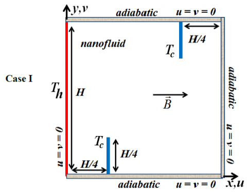
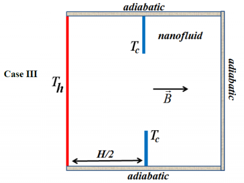
A two-dimensional square cavity with two heat sinks vertically attached to the horizontal walls is considered for the present study with the physical dimensions as shown in the Fig. 1. The temperatures Th and Tc< Thare uniformly imposed along the left vertical walls and the heat sinks. The right, top and bottom surfaces are assumed to be adiabatic. A magnetic field with uniform strength B0 is applied in the horizontal direction. The cavity is filled with water and Al2O3 nanoparticles. The nanofluid is Newtonian and incompressible. The flow is considered to be steady, two dimensional and laminar, and the radiation effects are negligible. The base fluid and the nanoparticles are in thermal equilibrium, the nanofluids were assumed to be similar to a pure fluid and then nanofluid qualities were calculated and they were applied for the equations of the considered problem. The thermo-physical properties of the base fluid and the nanoparticles are given in Table 1.
Table 1. Thermo-physical properties of water and nanoparticles
|
|
ρ (kg /m3) |
Cp (J/kg K) |
k (W/mK) |
β (K-1) |
|
Pure water |
997.1 |
4179 |
0.613 |
21x10-5 |
|
Al2O3 |
3970 |
765 |
40 |
0.85x10⁻⁵ |
The density variation in the nanofluid is approximated by the standard Boussinesq model. It is assumed that the induced magnetic field produced by the motion of an electrically conducting fluid is negligible compared to the applied magnetic field. Furthermore, it is assumed that the viscous dissipation and Joule heating are neglected. The classical models reported in the literature are used to determine the properties of the nanofluid:
$\rho_{n f}=(1-\phi) \rho_{f}+\phi \rho_{p}$(1)
$\left(\rho c_{p}\right)_{n f}=(1-\phi)\left(\rho c_{p}\right)_{f}+\phi\left(\rho c_{p}\right)_{p}$(2)
$(\rho \beta)_{n f}=(1-\phi)(\rho \beta)_{f}+\phi(\rho \beta)_{p}$(3)
$\alpha_{n f}=\frac{k_{n f}}{\left(\rho c_{p}\right)_{n f}}$(4)
In the above equations, $\phi$ is the solid volume fraction, ρ is the density, α is the thermal diffusivity, cp is the specific heat at constant pressure, k is the thermal conductivity and β is the thermal expansion coefficient. The viscosity of the nanofluid containing a dilute suspension of small rigid spherical particles and the thermal conductivity of the nanofluid can be modelled by [4]:
$\mu_{n f}=\frac{\mu_{f}}{(1-\phi)^{2.5}}$(5)
$k_{n f}=k_{f} \frac{k_{P}+2 k_{f}-2 \phi\left(k_{f}-k_{P}\right)}{k_{P}+2 k_{f}+\phi\left(k_{f}-k_{P}\right)}$(6)
For the incompressible non isothermal problems, Lattice Boltzmann Method (LBM) utilizes two distribution functions, f and g, for the flow and temperature fields respectively.
For the flow field:
$f_{i}\left(\mathbf{x}+\mathbf{c}_{\mathbf{i}} \Delta t, t+\Delta t\right)=f_{i}(\mathbf{x}, t)-\frac{1}{\tau_{v}}\left(f_{i}(\mathbf{x}, t)-f_{i}^{\mathrm{eq}}(\mathbf{x}, t)\right)+\Delta t F_{i}$(7)
For the temperature field:
$\mathrm{g}_{i}\left(\mathbf{x}+\mathbf{c}_{\mathbf{i}} \Delta t, t+\Delta t\right)=\mathbf{g}_{i}(\mathbf{x}, t)-\frac{1}{\tau_{\alpha}}\left(\mathrm{g}_{i}(\mathbf{x}, t)-\mathbf{g}_{i}^{\mathrm{eq}}(\mathbf{x}, t)\right)$(8)
where the discrete particle velocity vectors defined by ci ,$\Delta t$ denotes lattice time step which is set to unity. $\tau_{v}$, $\tau_{α}$ are the relaxation time for the flow and temperature fields, respectively.$f_{i}^{\mathrm{eq}}, \mathbf{g}_{i}^{\mathrm{eq}}$ are the local equilibrium distribution functions that have an appropriately prescribed functional dependence on the local hydrodynamic properties which are calculated with Eqs.(9) and (10) for flow and temperature fields respectively.
$f_{i}^{\mathrm{eq}}=\omega_{i} \rho\left[1+\frac{3\left(\mathbf{c}_{\mathrm{i}} \mathbf{u}\right)}{c^{2}}+\frac{9\left(\mathbf{c}_{\mathrm{i}} \mathbf{u}\right)^{2}}{2 c^{4}}-\frac{3 \mathbf{u}^{2}}{2 c^{2}}\right]$(9)
$\mathrm{g}_{i}^{\mathrm{eq}}=\omega_{i}^{\prime} T\left[1+3 \frac{\mathbf{c}_{\mathrm{i}} \cdot \mathbf{u}}{c^{2}}\right]$(10)
u and $\rho$ are the macroscopic velocity and density, respectively. c is the lattice speed which is equal to $\Delta x/ \Delta t$ where $\Delta x$ is the lattice space similar to the lattice time step $\Delta t$ which is equal to unity, $\omega_{i}$is the weighting factor for flow, $\omega_{i}^{\prime}$ is the weighting factor for temperature. D2Q9 model for flow and D2Q4 model for temperature are used in this work so that the weighting factors and the discrete particle velocity vectors are different for these two models and they are calculated with Eqs (11-13) as follows:
For D2Q9
$\omega_{0}=\frac{4}{9}, \omega_{i}=\frac{1}{9}$ for $i=1,2,3,4$ and $\omega_{i}=\frac{1}{36}$ for $i=5,6,7,8$(11)
The discrete velocities for the D2Q9 are defined as follows:
$\mathbf{c}_{\mathbf{i}}=\left\{\begin{array}{rl}{0} & {i=0} \\ {(\cos [(i-1) \pi / 2], \sin [(i-1) \pi / 2]) c} & {i=1,2,3,4} \\ {\sqrt{2}(\cos [(i-5) \pi / 2+\pi / 4], \sin [(i-5) \pi / 2+\pi / 4]) c} & {i=5,6,7,8}\end{array}\right.$ (12)
For D2Q4
The temperature weighting factor for each direction is equal to$\omega_{i}^{\prime}=1 / 4$ . The discrete velocities for the D2Q4 are defined as follows:
$\mathbf{c}_{\mathrm{i}}=(\cos [(i-1) \pi / 2], \sin [(i-1) \pi / 2]) c \quad i=1,2,3,4$(13)
The kinematic viscosity ν and the thermal diffusivity α are then related to the relaxation time by Eq. (14):
$v=\left[\tau_{v}-\frac{1}{2}\right] c_{s}^{2} \Delta t \qquad \alpha=\left[\tau_{\alpha}-\frac{1}{2}\right] c_{s}^{2} \Delta t$(14)
where cs is the lattice speed of sound witch is equals to $c_{s}=c / \sqrt{3}$. In the simulation of natural convection, the external force term F appearing in Eq. (7) is given by Eq.(15)
$F_{i}=\frac{\omega_{i}}{c_{s}^{2}} F \cdot c_{i}$(15)
$F=-\frac{H a^{2}}{H^{2}} \frac{\sigma_{n f}}{\sigma_{f}} \mu_{f} v+(\rho \beta)_{n f} g_{r}\left(T-T_{m}\right)$(16)
with
$H a=H B_{0} \sqrt{\frac{\sigma_{f}}{\mu_{f}}}$(17)
σ is the electrical conductivity.
$\sigma_{n f}=(1-\phi) \sigma_{f}+\phi \sigma_{p}$(18)
The macroscopic quantities, u and T can be calculated by the mentioned variables, with Eq.(19-21).
$\rho=\sum_{i} f_{i}$(19)
$\rho \mathbf{u}=\sum_{i} f_{i} \mathbf{c}_{i}$(20)
$T=\sum_{i} \mathrm{g}_{i}$(21)
2.1 Non dimensional parameters
By fixing Rayleigh number, Prandtl number and Mach number, the viscosity and thermal diffusivity are calculated from the definition of these non dimensional parameters.
$v_{f}=N . M a . c_{s} \sqrt{\frac{\operatorname{Pr}}{\mathrm{Ra}}}$(22)
where N is number of lattices in y-direction. Rayleigh and Prandtl numbers are defined as:
$R a=\frac{g_{r} \beta_{f} H^{3}\left(T_{h}-T_{c}\right)}{v_{f} \alpha_{f}}$ $\operatorname{Pr}=\frac{v_{f}}{\alpha_{f}}$(23)
Mach number should be less than $M a=0.3$ to insure an incompressible flow. Therefore, in the present study, Mach number was fixed at$M a=0.1$. The local Nusselt number and the average value at the left wall are calculated as:
$\mathrm{Nuy}=-\frac{k_{n f}}{k_{f}} \frac{H}{\mathrm{T}_{\mathrm{h}}-\mathrm{T}_{\mathrm{c}}}\left.\frac{\partial T}{\partial x}\right|_{\mathrm{x}=0}$(24)
$\mathrm{Nu}=\frac{1}{H} \int_{0}^{H} \mathrm{Nuydx}$(25)
$\mathrm{Nu}^{*}=\frac{\mathrm{Nu}(\varphi)}{\mathrm{Nu}(\varphi=0)}$(26)
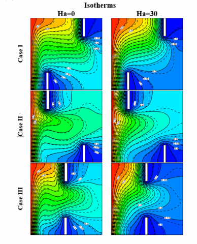
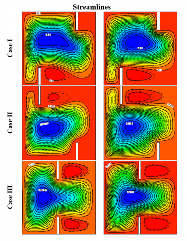
Fig.2 shows the effect of the Hartmann number and the Rayleigh number, on the isotherms and the streamlines of nanofluid ($\phi$=0.04) and pure fluid ($\phi$=0) for three different placement configurations of the heat sinks. The streamlines show, for all Hartmann number, a big cell in clockwise rotation is formed inside the cavity. The presence of heat sinks produces inactive areas next to the right vertical wall. These inactive areas are larger in case III. Isotherms show that inactive areas correspond to cold areas. For the case I and II, an intense temperature gradient appears between the hot wall and the cold source, indicating strong heat transfer rate in this region. The positions of the heat sinks greatly influence the nanofluid temperature. For the case I, the cold zone is located at the bottom of the cavity next to cold wall, for the case II the cold zone is located at the top of the cavity next to cold wall and for the case III, the cold zone is located in the right half of the cavity next to the right wall. The position and the size of these cold zones influence the flow intensity in the cavity.
Figure 2. Isotherms and streamlines Ra = 105 for (¯¯¯) $\Phi$= 0.04 and (- - -) $\Phi$= 0
Figure 3. Variation of the stream function maximum with (a) Hartmann number (Ra=105) (b) Rayleigh number (Ha=30) for $\Phi$= 0
Fig.3a and b show the variation of the stream function maximum respectively depending on Hartman number (Ra=105) and Rayleigh number (Ha=30) for $\phi$=0. For the three cases studied, the results show that the effect of Hartmann number is opposite to the effect of Rayleigh number. The stream function maximum increases with the increase of Rayleigh number and decreases with the rise of Hartmann number. The lowest intensity of the flow is obtained for the case I, whereas the flow intensity is almost the same for the other two cases. Thus, the positions of the heat sinks influence the flow intensity by the modification of the temperature distribution in the cavity.
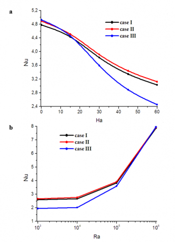
Fig.4a and b show the variation of the average Nusselt number along the hot wall respectively depending on Hartman number (Ra=105) and Rayleigh number (Ha=30) for $\phi$=0. For the three cases studied, the results show that the heat transfer rate increases with the increase of Rayleigh number and decreases with the increase of Hartmann number. Fig.4a show that for Ha < 15 the heat transfer rate is almost the same for the three cases studied. For Ha > 15, the lowest heat transfer rate is obtained for the case III, whereas the heat transfer rate is almost the same for the other two cases. For the case III, relative to the other cases, the heat sinks positions are far from the hot vertical wall, which explains the low heat transfer rate exchanged for the case III. Fig.4b show that for Ra < 105 the lowest heat transfer rate is obtained for the case III, while for Ra > 105 the heat transfer rate is almost the same for the three cases studied. Fig.4a and b indicates that the case I and II give the same average heat transfer rate along the hot wall.
Figure 4. Variation of the average Nusselt number with (a) Hartmann number (Ra=105) (b) Rayleigh number (Ha=30) for $\Phi$= 0
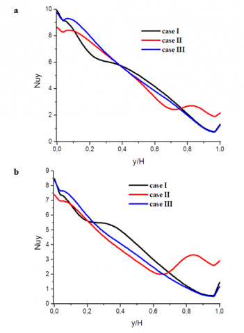
Figure 5. Variation of the local Nusselt number for Ra = 104 and $\Phi$= 0 for (a) Ha = 0 (b) Ha=30
Fig.5a and b show the local Nusselt number along the hot wall for Ra=104, $\phi$= 0 and respectively Ha=0 and 30. The results show that the Nusselt number greatly affects heat transfer rate. For cases I and III, the heat transfer occurs mainly at the bottom of the hot wall. Whereas for case II, for Ha =0, the average Nusselt number takes the same value at the bottom and the top of the hot wall, the minimum heat transfer rate is produced in the middle of the wall. The Hartmann number opposes the effect of Rayleigh number and greatly influences the heat transfer rate in case II.
Figure 6. Variation of the local Nusselt number for Ra = 105 and $\Phi$= 0 for (a) Ha =0 (b) Ha=30
Fig.6a and b show the local Nusselt number along the hot wall for Ra=105, $\phi$= 0 and respectively Ha=0 and 30. The results show that for high Rayleigh numbers, the local Nusselt number has almost the same shape for the three studied cases. The heat transfer rate is produced mainly at the lower half of the hot wall. Also, the magnetic field tends to reduce the heat transfer rate.
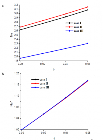
Fig.7 shows the effects of volume fractions on the average Nusselt number and the dimensionless average Nusselt number for Ra=103 and Ha=0. For the three studied cases, the heat transfer increases with the rise of volume fraction. The biggest heat transfer rate is obtained for case II and the dimensionless average Nusselt number has the same values for the three cases.
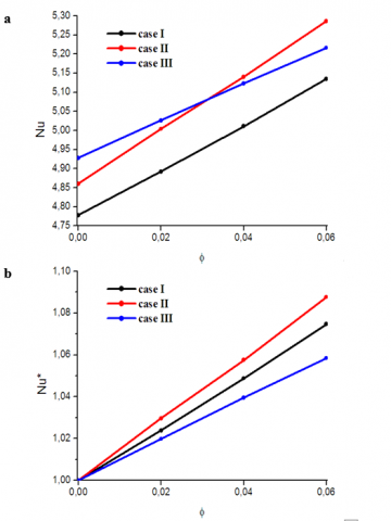
Fig.8 shows the effects of volume fractions on the average Nusselt number and the dimensionless average Nusselt number for Ra=105 and Ha=0. The lower heat transfer rate is obtained for case I. for $\phi$< 0.03, the greater heat transfer rate is obtained for case III, while $\phi$> 0.03 it is obtained for case II. The most significant effect of nanoparticles is obtained for case II.
Figure 7. Variation of the (a) average Nusselt number and (b) dimensionless average Nusselt number with $\Phi$ for Ra = 103 and Ha = 0
Figure 8. Variation of the (a) average Nusselt number and (b) dimensionless average Nusselt number with $\Phi$ for Ra = 105 and Ha = 0
Fig.9 shows the effects of volume fractions on the average Nusselt number and the dimensionless average Nusselt number for Ra=105 and Ha=30. For the three studied cases, the heat transfer increases with the rise of volume fraction. The greater heat transfer rate and the most significant effect of nanoparticles are obtained for case II. Also, the lower heat transfer rate and nanoparticles effect are obtained for case III. The behavior of nanoparticles depends strongly on the heat sinks positions.
Figure 9. Variation of the (a) average Nusselt number and (b) dimensionless average Nusselt number with $\Phi$ for Ra = 105 and Ha =30
In this paper the effects of the heat sinks, Rayleigh number, Hartmann number and solid volume fraction has been analyzed with Lattice Boltzmann Method. For the different configurations of the heat sinks, this study has been carried out for the pertinent parameters in the following ranges: Rayleigh number of the base fluid, Ra=103–105, Hartmann number between 0 and 60 and solid volume fraction from $\phi$=0 to 0.06. This investigation was performed for various mentioned parameters and some conclusions were summarized as follows:
|
B c cs ci cp F f f eq g geq gr H Ha k Ma Nu Pr Ra T |
Magnetic field (Tesla) Lattice speed (ms-1) Speed of sound (ms-1) Discrete particle speeds (ms-1) Specific heat at constant pressure (JK-1) External forces (kg m s-2) Density distribution functions (kgm-3) Equilibrium density distribution functions (kgm-3) Internal energy distribution functions (K) Equilibrium internal energy distribution (K) Gravity vector (m s-2) cavity length (m) Hartmann number thermal conductivity (Wm-1K-1) Mach number Local Nusselt number Prandtl number Rayleigh number Temperature (K) |
Greek symbols
|
τα τν υ α ρ σ ψ Ф |
Relaxation time for temperature (s) Relaxation time for flow (s) Kinematic viscosity (m² s-1) Thermal diffusivity (m² s-1) Fluid density (kgm-3) electrical conductivity (Ω-1 m-1) Non-dimensional stream function Solid volume fraction |
[1] S. N. Singh and D. K. Singh, “Study of combined free convection and surface radiation in closed cavities partially heated from below,” International Journal of Heat and Technology, vol. 33 (2), pp. 1-8, 2015. DOI: 10.18280/ijht.330201.
[2] F. Corvaro, G. Nardini, M. Paroncini and R. Vitali, “PIV and numerical analysis of natural convective heat transfer and fluid flow in a square cavity with two vertical obstacles,” International Journal of Heat and Technology, vol. 33 (2), pp. 51-56, 2015. DOI: 10.18280/ijht.330208.
[3] I. Mejri, A. Mahmoudi, M. A. Abbassi and A. Omri. (2014, March). Lattice Boltzmann simulation of conduction-radiation heat transfer in a planar medium. International Journal of Heat and Technology. [Online]. vol. 32 (1), pp. 213–218. Availabe: http://www.iieta.org/Journals/H%26TECH/ARCHIVE/Volume%2032%20No%201-2.
[4] I. Mejri and A. Mahmoudi, “MHD natural convection in a nanofluid-filled open enclosure with a sinusoidal boundary condition,” Chemical Engineering Research and Design, vol. 98, pp. 1-16, 2015. DOI: 10.1016/j.cherd.2015.03.028.
[5] I. Mejri, A. Mahmoudi, M. A. Abbassi and A. Omri, “Magnetic field effect on entropy generation in a nanofluid-filled enclosure with sinusoidal heating on both side walls,” Powder Technol., vol. 266, pp. 340-353, 2014. DOI: 10.1016/j.powtec.2014.06.054.
[6] I. Mejri, A. Mahmoudi, M. A. Abbassi and A. Omri, “MHD natural convection in a nanofluid-filled enclosure with non-uniform heating on both side walls,” Fluid Dynamics and Materials Processing, vol. 10, pp. 83–114, 2014. DOI: 10.3970/fdmp.2014.010.083.
[7] I. Mejri, A. Mahmoudi, M. A. Abbassi and A. Omri, “Magnetic field effect on natural convection in a nanofluid filled enclosure with non-uniform heating on both side walls,” International Journal of Heat and Technology, vol. 32, pp. 127-133, 2014. http://www.iieta.org/Journals/H%26TECH/ARCHIVE/Volume%2032%20No%201-2.
[8] I. Mejri, A. Mahmoudi, M. A. Abbassi and A. Omri, “Lattice Boltzmann simulation of MHD natural convection in a nanofluidfilled enclosure with non-uniform heating on both side walls.” in IEEE Xplore, Composite Materials & Renewable Energy Applications (ICCMREA), 2014 International Conference, Sousse, 2014, pp. 1-5. DOI: 10.1109/ICCMREA.2014.6843797.
[9] A. Mahmoudi, I. Mejri, M. A. Abbassi and A. Omri, “Lattice Boltzmann simulation of MHD natural convection in a nanofluid-filled cavity with linear temperature distribution,” Powder Technology, vol. 256, pp. 257–271, 2014. DOI: 10.1016/j.powtec.2014.09.022.
[10] A. Mahmoudi, I. Mejri, M. A. Abbassi and A. Omri. (2014, March). Lattice Boltzmann simulation of magnetic field direction effect on natural convection of nanofluid-filled cavity. International Journal of Heat and Technology. [Online]. vol. 32 (1), pp. 9-14. Available: http://www.iieta.org/Journals/H%26TECH/ARCHIVE/Volume%2032%20No%201-2.
[11] A. Mahmoudi, I. Mejri, M. A. Abbassi and A. Omri, “Lattice Boltzmann simulation of MHD natural convection in a nanofluid-filled cavity with linear temperature distribution,” in IEEE Xplore, Composite Materials & Renewable Energy Applications (ICCMREA), 2014 International Conference, Sousse, 2014, pp. 1-4. DOI: 10.1109/ICCMREA.2014.6843796.
[12] A. Mahmoudi, I. Mejri, M. A. Abbassi and A. Omri, “Analysis of the entropy generation in a nanofluid-filled cavity in the presence of magnetic field and uniform heat generation/absorption,” Journal of Molecular Liquids, vol. 198, pp. 63–77, 2014. DOI: 10.1016/j.molliq.2014.07.010.
[13] A. Mahmoudi, I. Mejri and A. Omri, “Study of natural convection cooling of a nanofluid subjected to a magnetic field,” Physica A, vol. 451, pp. 333-348, 2016. DOI: 10.1016/j.physa.2016.01.102.
[14] A. Mahmoudi, I. Mejri, M. A. Abbassi and A. Omri, “Numerical study of natural convection in an inclined triangular cavity for different thermal boundary conditions: application of the lattice Boltzmann method,” Fluid Dynamics and Materials Processing, vol. 9, pp. 353-388, 2013. DOI: 10.3970/fdmp.2013.009.353.