OPEN ACCESS
In this paper, an approach is proposed for measuring three-dimensional (3D) turbulence velocities by the vector characteristics of flow velocity. Based on the principle of vector decomposition and synthesis, a special multi-vector three components (3C) tripod structure, which can sense flow velocities with little disturbance to the measured flow, is studied. At the front most of the 3C structure, the sensing ball exposed to the flow creates strains on each of the three silicon piezoresistance beams, and the corresponding deformation of the beams is converted into electrical output signals by the Wheatstone bridge. The desired 3D turbulent velocities could be obtained by the vectors output signals of the three piezoresistive sensing microcircuits with an embedded microprocessor. The reasonability and feasibility of the 3D structure design can be verified by simulation experiments. The 3D velocities data can be collected in a certain period of time in a transparent water experiment. Furthermore, this method as a complex way will be used for measuring 3D turbulence velocity in fluid flow with hyper-sediment content up to 350kg/m3, where the Laser Doppler Velocimeter (LDV) and other types of flow meter cannot be used.
Three-dimensional turbulence velocity, Vector decomposition and synthesis, Piezoresistance, Laser Doppler Velocimeter (LDV).
Study on the turbulence velocity and intensity distribution structure of a fluid flow containing sediment is essential original conductive research of natural river dynamics in a lab [1-2]. It mainly depends on development of measurement techniques and the authenticity and accuracy of historical turbulence records during experiments to understand the fluid flow turbulence velocity. Throughout the development of the current velocimeter (turbulence velocity measurement in sediment content flow), a silicon piezoresistance velocity meter and Laser Doppler Velocimeter (LDV) which could be used only in very low sediment content flow are widely used. The former adopts the intrusive contact measurement and could be used in hyper-sediment flow under conditions with a certain acceptable interference to the flow and needs to be a dedicatedly designed and manufactured shape and size to minimize error. Meanwhile, the transducer also must be calibrated by a specially designed calibration system to make its outputs strictly correspond to the flow in a layer flow situation, and the pipe pulse jet flow calibration must be set to calibrate its resonant frequency in order to ensure its dynamic performance [3-4]. LDV adopts a non-contact measurement method that could only be used in transparent water flow or very low sediment content flow, but not hyper sediment content fluid [5-6].
As is known, Acoustic Doppler Velocimeter (ADV) is another intrusive transducer used to measure flow velocity [7-8], but ultrasonic sensors could not precisely identify the flow or water movement due to the echoed sound intermittently coming from a complex flow unit, and regularly the size and shape disturbed the flow too much.
PIV is often used for the validation of Reynolds-averaged Navier–Stokes (RANS) computations and the study of high Reynolds number flows where the direct numerical simulation (DNS) of the governing equations is not feasible [9-10].
It has been a bottleneck to measure three-dimensional turbulence velocity in flow with hyper-sediment content for many years since 1989 [11-12] due to the two features of the hyper sediment content fluid flow: (1) non-transparence, which hinders the use of LDV and the feature, and (2) concessional disturbance to the flow, which makes it difficult to find a structure as an intrusive transducer to sense the 3D flow velocity within an acceptable sensor size and shape. Until now it has been a puzzle to find a structure to design the transducer [12]. Meanwhile, the above measurement equipment are mostly used for one-dimensional and two-dimensional turbulence velocity measurement of the flow. The reason why there is a limitation for measuring 3D turbulence flow is that the precision of the volume of the sensing unit and the sensitivity of the sensor are so strictly required. The sensing part is the soul of a transducer which converts the measured physical information to electronic signals. A well-known method to measure turbulence velocity is directly sensing the flow force, which had been practiced since the 1950’s [13-14] until the time the 2D sensor was designed and tested in the sediment content fluid flume in The State Key Laboratory of Water Resources and Hydropower Engineering Science, Wuhan University in 1995 [15-16]. But it has been difficult to measure three-dimensional velocity in sediment flow due to the need for an intrusive sensor of a certain precise size and shape to keep the extra turbulence created by the transducer to an acceptable level of error [17-18].
In this paper, an innovative 3C tripod structure is designed with a 3mm ball in the front of the structure which is exposed to the fluid. When the sensing ball is driven by the flow force, the corresponding flow velocities and the turbulent velocities could be determined by pointing the vectors branches to the detecting direction from an embedded Wheatstone bridge. This method can be applied both in hyper-sediment flow and transparent water flow to measure turbulence. The new type of 3D turbulent velocity measurement system will be a device for studies of fluid mechanics, and will provide a new solution for the demand in the study of river dynamics.
2.1 Principle of velocity detection
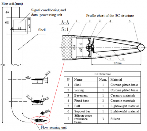
The 3C tripod structure is designed to adapt vector characteristics of flow, so as to be able to sense each of the velocity vectors by a silicon piezoresistance beam as shown in Figure 1. The flow sensing ball is 3 mm in diameter and the core of the ball is the meeting point of the three vector support bars. The other end of each tripod bar is spliced to one end of the strain sensing silicon piezoresistance beam that measures the vector pressure of the bar in the direction of the flow. The other ends of the silicon beam of each of the tripod bars are spliced to the ceramic support base by low temperature glass. Once the ball is exposed to flow, the velocity of the flow creates strains on the sensing parts which converted the strains into electrical output signals by the Wheatstone bridge of the signal conditioning unit. The signal conditioning unit (as shown in Figure 7) is a multi-vector processing apparatus, in which the measured 3C vectors can be synthesized to the flow turbulence velocities’ directions corresponding to the vectors which represent the turbulence velocities of the flow, and they are longitudinal velocity, vertical velocity, horizontal velocity, denoted as $u$, $v$, $w$.
Figure 1. 3C tripod sensing structure
Since the silicon piezoresistance beam is made of highly rugged material and the force created by the flow in flume is quite small, the deformation in the silicon piezoresistance beams could go undetected in analysis. The changes in resistivity of the piezoresistance are dominated by strain caused by the front ball and the tripod bars. The detecting 3C structure is a vibration free system and the beam curve angle is small in order to keep the transducer shell profile size as small as possible. The relationship between the force of the external flow and the angle could be taken as a linear relationship [15] .The vibrating differential equation of the system can be described as:
$m \frac{d^{2} x}{d t^{2}}+c \frac{d x}{d t}+k x=F(t)$ (1)
Let $k / m=\omega_{p}^{2}, c / m=2 D$ , and Formula 1 can be rewritten as:
$\frac{d^{2} x}{d t^{2}}+2 D \frac{d x}{d t}+\omega_{p}^{2} x=F(\mathrm{t})$ (2)
Where $m$ is the mass of the beam and the relative structure materials, $c$is the resistivity coefficient and $k$ is the elastic coefficient, $\omega_{p}$ is the systematic free vibrating radian frequency, $D$ is the attenuation coefficient.
The turbulence flow is not periodic, but within a relatively long period of time, and the average turbulence velocities in both vertical and horizontal direction of a flume could be thought of as zero. In a given time period, the portion of turbulence velocity is made of multi-harmonic waves and is considered as the excitation of the system, described as follows:
$F(\mathrm{t})=\sum_{i=0}^{n} F_{i} \sin \left(\omega_{i} t+\varphi_{i}\right)$ (3)
Where n is the highest frequency in the turbulence flow, $F_{i}$ is the amplitude of the force, $\varphi_{i}$ is the phase angle, and $\omega_{i}$ is the flow radian frequency acting on the transducer. Normally $\omega_{i}$ is less than 100 Hz in the lab’s fluid flow flume where the average velocity of sediment content fluid flow is less than 3m/s, meanwhile, and n decreases as the sediment content increases. As seen in Formulas 2 and 3, the general solution equation of the system could be to say:
$\begin{aligned} x(t)=& e^{-D t}\left(C_{1} e^{t \sqrt{D^{2}-\omega_{p}^{2}}}+C_{2} e^{-t \sqrt{D^{2}-\omega_{p}^{2}}}\right) +\sum_{i=1}^{n} X_{i} \sin \left(\omega_{i} t+\phi_{i}\right) \end{aligned}$ (4)
In the above equation, the first part is a free vibration function of the system, which is a fast diminishing one. The second part represents the forced vibration of the system when the sensor is excited by the flow. In a linear system, it is thought of as corresponding to the acting force. With a suitable silica gal filler damper in the 3C structure tube, the resonant vibration of the sensor should be higher than 500 Hz, as indicated by the pulse jet calibration test, which matches the frequency response demand of the turbulence measurement.
2.2 Principle of vector decomposition and synthesis
The force analysis in three-dimensional space is shown in Figure 2. The angle between each support bar and the centricity of the tripod is $\theta$. In the preliminary design, $\theta$ is 10° to fit the size demand of the transducer. The angle between two of any of the three fixed support bars is 120°. The angle between any of the three support bars and the silicon piezoresistance beams is 90° to keep a good linearity signal conditioning of the Wheatstone bridge, as shown in Figure 3.
Figure 2. Force analysis of 3C structure for velocity detection
Let $\vec{f}$denote the force (F) acting on the target bar. Let$f_{1}$, $f_{2}$ and $f_{3}$ denote the magnitude of the forces acting on the support bars. The direction of the forces is along the support bars. According to the decomposition and synthesis principle of vectors, the force of each support bar can be decomposed in x, y, z directions as follows.
(1) Bar 1’s branch force
$f_{x}^{1}=f_{1} \sin \theta, f_{y}^{1}=0, f_{z}^{1}=f_{1} \cos \theta$ (5)
(2) Bar 2’s branch force
$f_{x}^{2}=-f_{2} \sin \theta \cos 60^{\circ}$ ,
$f_{y}^{2}=f_{2} \sin \theta \sin 60^{\circ}$ ,
$f_{z}^{2}=f_{2} \cos \theta$ (6)
(3) Bar 3’s branch force
$f_{x}^{3}=-f_{3} \sin \theta \cos 60^{\circ}$ ,
$f_{y}^{3}=-f_{3} \sin \theta \sin 60^{\circ}$ ,
$f_{z}^{3}=f_{3} \cos \theta$ (7)
Set: $H=\left[f_{x}, f_{y}, f_{z}\right]$ ,
$A=\left[f_{1}, f_{2}, f_{3}\right]$ ,
$B=\left(\begin{array}{ccc}\sin \theta & 0 & \cos \theta \\ -\sin \theta \cos 60^{\circ} & \sin \theta \sin 60^{\circ} & \cos \theta \\ -\sin \theta \cos 60^{\circ} & -\sin \theta \sin 60^{\circ} & \cos \theta\end{array}\right)$ ,
Then, $\vec{f}$ along x, y, z directions’ force $f_{x}$ , $f_{y}$ , $f_{z}$ can be calculated as follows.
$H=A^{*} B$ (8)
According to the Bernoulli Equation of fluid mechanics, in the flow of the lab’s flume (the flume is 33 m long, 0.5m width, 0.5m height, flow is controlled by valves between 3cm/s-3m/s), kinetic energy ($f$) of the fluid is proportional to the square of velocity ($v^{2}$) and fluid density ($\rho$), which can be simply expressed as:
$f \propto \rho|\vec{v}|^{2}$ (9)
According to the above analysis, the instant fluid velocity could be expressed as:
$|\vec{v}|=Q_{m} \sqrt[4]{f_{x}^{2}+f_{y}^{2}+f_{z}^{2}}$ (10)
In equations 9 and 10, $f=\vec{f} |=\sqrt{f_{x}^{2}+f_{y}^{2}+f_{z}^{2}}$ , $Q_{m}$ can be obtained by a calibration experiment of the transducer [13], where $\vec{v}$ and $\vec{f}$ have the same vector direction. Therefore, the longitudinal velocity, vertical velocity and horizontal velocity ($u$, $v$, $w$) can be expressed respectively as follows.
$u=v_{z}=|\vec{v}| \frac{f_{z}}{\sqrt{f_{x}^{2}+f_{y}^{2}+f_{z}^{2}}}$ (11)
$v=v_{x}=|\vec{v}| \frac{f_{x}}{\sqrt{f_{x}^{2}+f_{y}^{2}+f_{z}^{2}}}$ (12)
$w=v_{y}=|\vec{v}| \frac{f_{y}}{\sqrt{f_{x}^{2}+f_{y}^{2}+f_{z}^{2}}}$ (13)
With a series of measurements of the velocities in a time interval, the series data could be described as $\{u\}$ , $\{v\}$ , $\{w\}$ . The velocities of each direction and respective turbulence velocities can be calculated by above analysis.
2.3 Principle of strain measurement by silicon piezoresistance beam
The 3C structure with three silicon piezoresistance beams as the sensing element to detect the three different directions velocity vectors is the critical element of the transducer. The various strains on the 3C structure are converted to electrical output signals by Wheatstone bridges which are integrated into the silicon beams with the electronic signal processing unit [19-20]. The sketch map of the piezoresistances on a silicon beams is shown in Figure 3. The detection circuit of the three-dimensional velocity by each Wheatstone bridge is shown in Figure 4. With a suitable exciting constant current source, relative differential signal conditioning and filter circuits, the flow velocity can be measured.
Figure 3. Arrangement of piezoresistances on silicon beam
Figure 4. Wheatstone bridge circuits to detect force
According to the measurement principle of Wheatstone bridges, once the silicon beam detects the stress $f_{i}$ (that is $f_{1}$ , or $f_{2}$ , or $f_{e}$ ) from the support bar in one direction, the piezoresistances R2, R4 will increase, while R1, R3 will decrease. The larger the stress acting on the beam, the larger the output $U_{0}$ of the Wheatstone bridge. The relationship between the output voltage $U_{0}$ and the stress $f_{i}$ can be expressed as:
$U_{o}=\frac{4 \mu R_{2}^{0} R_{4}^{0}}{R_{1}+R_{2}+R_{3}+R_{4}} I_{a} \bullet f_{i}$ (14)
or
$U_{O}=\frac{4 \mu R_{1}^{0} R_{3}^{0}}{R_{1}+R_{2}+R_{3}+R_{4}} I_{a} \bullet f_{i}$ (15)
In Formulas 14 and 15, $I_{a}$ is the value of the exciting constant current source, $R_{1}^{0}$ , $R_{2}^{0}$ , $R_{3}^{0}$ , $R_{4}^{0}$ is the initial value of each silicon piezoresistance, $\mu$ is a constant corresponding to the bridge sensitivity to the applied force or the flow velocity. Wherein, $\mu=K \frac{\sigma_{i}}{E}$ ( $\sigma_{i}=\frac{f_{i}}{S}$ , $\sigma_{i}$ is strain force of silicon beam, S is the force area of silicon piezoresistanes, E is the elastic modulus, K is a strain sensitivity coefficient of silicon piezoresistanes) .
In order to improve the measurement sensitivity of the silicon piezoresistive effect, a finite element method (FEM) is used to analyze the stress distribution of the force and deformation of the elastic cantilever [21-22]. The finite element model is established by ANSYS software, in which N-type silicon is chosen as the support base, elastic modulus E take 130Gp, poison ratio is 0.278, parameters of beams are 450$\mu m$*150$\mu m$*50$\mu m$. The strain force ($\sigma_{i}$) distribution on the cantilever silicon beam under the action of corresponding stress force is shown in Figure 5. Owing to the difference of the strain distribution on each beam, combined with the measurement characteristic of the Wheatstone bridge, the measurement accuracy of each direction can be distinguished and improved .
Figure 5. Stress distribution on the three silicon beam
Figure 6 shows the structural design of the 3D turbulence velocity transducer in accordance with the improved measurement method put forward above. It is composed of three parts, and the appearance of the transducer will be shown in Figure 15.
Figure 6. Structural design of transducer
The first part is the flow sensing unit (called 3C tripod sensing structure) in the front of the main body. The front ball is the only part of the transducer exposed to the flow as the velocities sensing element is only 3mm in diameter to avoid affecting the frequency response of the transducer [23]. As the ball is mounted on the top of the tripod, and while the three bars together support the ball and guide the flow force caused by the flow velocity to the silicon beams in a rugged appropriately shaped metal shell, the integrated Wheatsone bridges on the corresponding silicon beam on the structure convert the flow velocities into electronic signals.
The second part is the main body which protects the sensor and signal conditioning unit. It consists of a 70 cm bronze knife-shaped shell with a sharp front designed to reduce the impact of the transducer on the original flow. At the top of main body is a square base designed to keep the transducer fixed during the test of flow to the support of the flume. The main body helps to fix the transducer and can be mounted on the flume to isolate the external disturbance and vibrations.
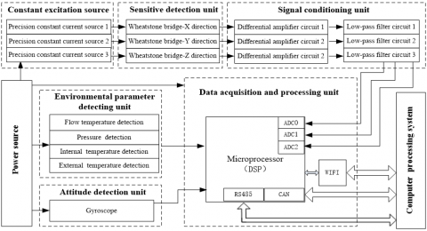
The third part is a box under the fixed base containing the signal conditioning unit and high speed data acquisition and processing unit. It is another critical part of the transducer where all the parameters are measured and processed simultaneously, so it is also called sensor measuring system. The circuit diagram is shown in Figure 7. This unit contains the transducer excitation source, output signals conditioning equipment including three-channel high-stability accurate signal amplifiers and the DSP processor as well as AD convertors, signal filter and digital vectors conversion function parts. Meanwhile, as turbulence flow is also impacted by many ambient factors, the sediment content flow’s temperature, laboratory’s ambient temperature and barometric pressure must also be measured for the system drift compensation. This complex transducer-conditioning-unit gives the final digital output with RS485 interface and a Wi-Fi wireless interface to connect for computer or app of a mobile device where all the measurement parameters can be set according to the transducer calibration result and get the order from mobile phone app to start a round of measurement.
Figure 7. Circuit diagram of high speed data acquisition and processing system
Table 1. The data for force’decomposition and synthesis
|
F |
F=0.056N |
F=0.112N |
F=0.140N |
||||||||||
|
β |
f1 (N) |
f2 (N) |
f3 (N) |
f1 (N) |
f2 (N) |
f3 (N) |
f1 (N) |
f2 (N) |
f3 (N) |
||||
|
15º |
0.1129 |
0.0898 |
0.1054 |
0.2259 |
1.7968 |
0.2109 |
0.2824 |
0.2246 |
0.2636 |
||||
|
30º |
0.1053 |
0.0809 |
0.0907 |
0.2105 |
0.1618 |
0.1813 |
0.2632 |
0.2022 |
0.2266 |
||||
|
45º |
0.0905 |
0.0667 |
0.0698 |
0.1809 |
0.1335 |
0.1395 |
0.2262 |
0.1668 |
0.1744 |
||||
|
60º |
0.0695 |
0.0486 |
0.0443 |
0.1392 |
0.0973 |
0.0886 |
0.1740 |
0.1216 |
0.1108 |
||||
|
90º |
0.0167 |
0.0167 |
0.0167 |
0.0334 |
0.0335 |
0.0333 |
0.0418 |
0.0418 |
0.0417 |
||||
|
|
F |
F=0.196N |
F=0.226N |
F=0.283N |
|||||||||
|
β |
f1 (N) |
f2 (N) |
f3 (N) |
f1 (N) |
f2 (N) |
f3 (N) |
f1 (N) |
f2 (N) |
f3 (N) |
||||
|
15º |
0.3953 |
0.3144 |
0.3690 |
0.4518 |
0.3593 |
0.4218 |
0.5647 |
0.4492 |
0.5272 |
||||
|
30º |
0.3685 |
0.2831 |
0.3173 |
0.4211 |
0.3235 |
0.3626 |
0.5264 |
0.4044 |
0.4533 |
||||
|
45º |
0.3167 |
0.2336 |
0.2442 |
0.3619 |
0.2669 |
0.2791 |
0.4524 |
0.3337 |
0.3489 |
||||
|
60º |
0.2435 |
0.1702 |
0.1551 |
0.2783 |
0.1946 |
0.1773 |
0.3479 |
0.2432 |
0.2216 |
||||
|
90º |
0.0585 |
0.0585 |
0.0583 |
0.0668 |
0.0669 |
0.0666 |
0.0836 |
0.0836 |
0.0833 |
||||
|
|
F |
F=0.339N |
F=0.453N |
F=0.509N |
|||||||||
|
β |
f1 (N) |
f2 (N) |
f3 (N) |
f1 (N) |
f2 (N) |
f3 (N) |
f1 (N) |
f2 (N) |
f3 (N) |
||||
|
15º |
0.6777 |
0.5390 |
0.6326 |
0.9035 |
0.7187 |
0.8435 |
1.0165 |
0.8085 |
0.9489 |
||||
|
30º |
0.6316 |
0.4853 |
0.5439 |
0.8422 |
0.6470 |
0.7252 |
0.9474 |
0.7279 |
0.8159 |
||||
|
45º |
0.5428 |
0.4004 |
0.4186 |
0.7238 |
0.5339 |
0.5582 |
0.8142 |
0.6006 |
0.6279 |
||||
|
60º |
0.4175 |
0.2918 |
0.2659 |
0.5566 |
0.3891 |
0.3545 |
0.6262 |
0.4378 |
0.3988 |
||||
|
90º |
0.1003 |
0.1004 |
0.1001 |
0.1337 |
0.1338 |
0.1333 |
0.1504 |
0.1505 |
0.1499 |
||||
4.1 Validation of forces’ decomposition and synthesis
According to the design of the transducer structure, the force will be automatically decomposed into three components along support bars when the flow sense ball is under impact of flow
fluid pressure. In order to verify the feasibility of the- 3C structural design and the principle of forces decomposition and synthesis, numerical analysis is given by the static stress analysis function module of Solidworks software. Examples provided are under assumptions that the transducer’s sensing ball (diameter of 3 mm) is placed in fluid flow, which is fully impacted by the measured flow. According to the Bernoulli Equation of fluid mechanics, the applying forces are set at a
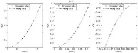
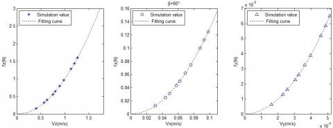
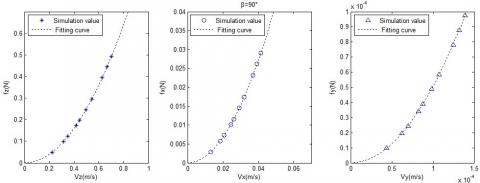
range from 0.05N to 0.5N, corresponding to the flow velocity from 0.5m/s to 3 m/s [24]. The forces ($f_{1}$, $f_{2}$, $f_{3}$) along three support beams are obtained through different placement angles ($\beta$) and different applying forces ($F$). In this experiment they are $\beta$=$15^{\circ}$ , $30^{\circ}$, $45^{\circ}$, $60^{\circ}$, $90^{\circ}$. The specific data is shown in Table 1. $f_{x}$ , $f_{y}$ , $f_{z}$ are the components of acting force $f$ in $x$, $y$ , $z$ directions which is shown in Figure 2. They are calculated based on the principle of decomposition and synthesis and the data is in Table 1. Thus $v_{x}$ , $v_{y}$ , $v_{z}$ can be obtained using the same method. The calculation results are curve fitting with the Matlab software, exactly as shown in Figure 8-(a), (b), (c), (d), (e).
(a)
(b)
(c)
(d)
(e)
Figure 8. The fitting curve $f_{z}$ and $\mathcal{V}_{z}$ , $f_{x}$ and $\mathcal{V}_{x}$ , $f_{y}$ and $\mathcal{V}_{y}$ in different placement angles
It can be seen in the above results, when $\beta$ = $15^{\circ}$ , $30^{\circ}$ , $45^{\circ}$ , $60^{\circ}$ , $90^{\circ}$ , $f_{z}$ and $v_{z}$ , $f_{x}$ and $v_{x}$ can be compared with $y=\xi x^{2}(\xi>0)$ curve fitting. when $\beta$ = $15^{\circ}$ , $30^{\circ}$ , $45^{\circ}$, $f_{y}$ and $v_{y}$ can be compared with $y=-\xi x^{2}(\xi>0)$ curve fitting. But when $\beta$ is $60^{\circ}$ or $90^{\circ}$ , $f_{y}$ and $v_{y}$ can be compared with$y=\xi x^{2}(\xi>0)$ curve fitting . This shows that when the $\beta$ < $45^{\circ}$ , the $f_{y}$ form the reaction force, the direction is opposite in $y$ direction, and on the other hand, $f_{y}$ and $v_{y}$ in the same direction.
Through the above analysis it can be speculated that $f_{x}$ , $f_{y}$ , $f_{z}$ and the corresponding $v_{x}$ , $v_{y}$ , $v_{z}$ can be fitted with $|y|=\xi x^{2}(\xi>0)$ curve when the transducer is placed at any angle. At the same time, as seen in Figure 9, the result verifies that the force ($F$) of fluid is proportional to the square of velocity ($v^{2}$). Proportional relations reflect a consistent linear relationship of the transducer, which is one of the most important characteristics of the transducer.
Figure 9. The relation F and V form the static stress analysis
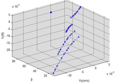
Because $v_{x}$ , $v_{y}$ , $v_{z}$ are related to longitudinal velocity, vertical velocity, horizontal velocity ($u$ , $v$ , $w$), the relationship between $f_{x}$ , $f_{y}$ , $f_{z}$and the corresponding $v_{x}$ , $v_{y}$ , $v_{z}$at different placement angles can be simulated in three-dimensional space as shown in Figure 10 (a), (b), (c) .
(a)X direction
(b)Y direction
(c)Z direction
Figure 10. The relationship between $f_{x}$ , $f_{y}$ , $f_{z}$and the corresponding $v_{x}$ , $v_{y}$ , $v_{z}$ at different placement angles in three-dimensional space
4.2 Characteristic analysis of transducer
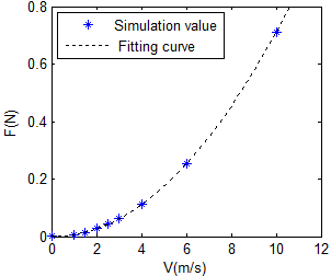
In this paper, the numerical simulation method is used for testing the relation between the force (F) and the velocity (V) by CFD. The numerical result is simulated by commercial code ANSYS Fluent 12.1. The standard k-ε model is adopted during simulation [25], and 2D axial-symmetric modeling is used in the simulating strategy. The calculating domain is shown in Figure 11 (a). The boundary condition of inlet and outlet, other than the wall, is velocity inlet and pressure outlet respectively. The mesh around the sensor is shown in Figure 11 (b) and the grid number is 50, 000.
Because the front ball is the only part of the transducer exposed to the flow, the knife-shaped shell with a sharp front was designed to reduce the impact of the transducer on the original flow. The vortex comparison between the single ball and the transducer in flow is shown in Figure 12. The vortex is created behind the ball when a single ball is derived by the flow. Because of the transducer shell’s shape, as seen in Figure 6, the front ball cannot sense the vortex at the tail of the 3C structure.
Figure 11. CFD model of the sensor
Figure 12. Vortex comparison between single ball and
transducer in flow
The relation between F and V is shown in Figure 13 as calculated by Fluent software. The relation curve between F and V can be fitted with $y=\xi x^{2}(\xi>0)$ curve, which verifies that the force ($F$) of fluid is proportional to the square of velocity ($v^{2}$).
Figure 13. Relation between F and V from the CFD
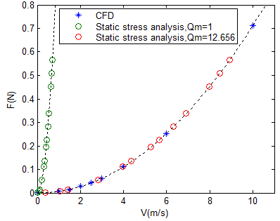
According to formula 10, assuming $Q_{m}$ =1, the V-F curve restults in that shown in Figure 14. The relationship between V-F could be formulated as $y=\xi x^{2}(\xi>0)$. The analysis using Matlab, where $Q_{m}$ =12.656, the relation curve between F-V from static stress analysis can match the relation curve between F-V from CFD perfectly as shown in Figure 14.
Figure 14. $Q_{m}$ theoretical calibration analysis
4.3 Result of measuring turbulent velocities
The transducer’s performance is studied in a flume, shown in Figure 15, which simulates a flume environment in The State Key Laboratory of Water Resources and Hydropower Engineering Science, Wuhan University, where the flume is 33m long, 0.5m width, 0.5m height. In the experiment, water depth varies from 5 to 30cm, flow velocity is between 3cm/s-3.5 m/s. the width of flow section is 1.2 m and the length of flow in 12m. With the depth of flow section being 0.16 m for example, five testing points are selected and their corresponding feature values are measured, results of which are shown in Table 2. The velocities data of $v_{x}$, $v_{y}$ and $v_{z}$ (in 0.6 h) is collected in 30 second periods as shown in Figure 16.
Figure 15. Measuring environment in laboratory flume
This experiment is carried out in transparent water by acquiring current velocities in a certain period of time continuously [26], then average of velocities is obtained. The whole experiment process, including data acquisition, data processing and data display, is completed by computers and the corresponding client app.
Table 2. Feature value of velocity measurement
|
Measuring point |
Maximum value V (m/s) |
Minimum value V (m/s) |
Average value V (m/s) |
Standard deviation |
|
0.8 h |
3.23 |
1.47 |
2.26 |
0.47 |
|
0.6 h |
3.06 |
1.21 |
2.12 |
0.45 |
|
0.4 h |
3.12 |
1.11 |
2.04 |
0.44 |
|
0.2 h |
3.00 |
1.06 |
1.88 |
0.42 |
|
0.1 h |
2.86 |
0.85 |
1.76 |
0.41 |
Figure 16. The velocities data of $v_{x}$ , $v_{y}$ and $v_{z}$ (0.6 h) in 30 seconds
As is shown above, the method is based on the elastic component whose natural frequency of vibration is above 100Hz and can measure three-dimensional turbulent velocity at the same testing point in a period of time. In the experiment, it is found that the flow turbulence can be well detected at a water depth of 0.1m when current average velocity is below 1.5m/s.
The innovative 3D turbulence velocity transducer structure is introduced in this paper. A systematic analysis validates the design of the three-dimensional 3C tripod structure. The principle of vector decomposition and synthesis is used in the measurement of 3D turbulence velocities (longitudinal velocity, vertical velocity, and horizontal velocity). The transducer can be used both in transparent water and in hyper-sediment content flow as a complementary method to complete the three dimensional velocity measurement in any flow where LDV is not suitable to use. At the same time, the structure can be used to make 3D measurement possible in sediment content flume test to study river dynamics. This advanced method provides a new detection technique for studying the basic theory of water flow structure to facilitate fluid mechanics study.
As a new structure and measuring method for three-dimensional turbulent velocities in fluid flow, much work remains for future research. The characteristics and error propagation of the transducer will be studied seriously in the following extended period of experiments using various sediment content and various velocities. Before each time of experiments, the transducer needs a systematic calibration in order to obtain valuable data for fluid dynamics study. So, the construction of 3D calibration station and hyper sediment content flow experiments will be key work in future.
This work is sponsored by the National Natural Science Foundation of China (Grant No. 61272114 and No. 41376022), Marine Renewable Energy Special Fund Project of the State Oceanic Administration of China (Grant No.GHME2013JS01), and the invention patent of China (Grant NO.201410240248.5)
In this work, Guilin Zheng focused on the principle of turbulent velocities measurement. Li Zhang (*Corresponding author) performed the force analysis of the pyramid structure in three-dimensional space and simulation experiments. Xiangtao Zhuan conducted analysis of transduce. All authors pecified the comparative study, and were involved in discussing the results and developing the final conclusions.
1. G.Q. Wang,“Advances in river sediment research,” Journal of Sediment Research,no.2,pp.64–81,2007.
2. S.Fukuoka,H. Nakagawa,T. Sumi,H. Zhang, Advances in River Sediment Research, CRC Press, Florida, 2013.
3. Lečić, M.R., Čantrak Đ.S., Ćoćić A.S. and Banjac, M.J., “Piezoresistant velocity probe,” Experimental Techniques, vol.33, no.3, pp.73-79, 2009. DOI: 10.1111/j.1747-1567.2008.00365.x.
4. Y. Su,A. Evans,A. Brunnschweiler,G. Ensell,“Characterization of a highly sensitive ultra-thin piezoresistive silicon cantilever probe and its application in gas flow velocity sensing,” Journal of Micromechanics and Microengineering,vol.12,no.l6,pp.1-6,2002.DOI: 10.1088/0960-1317/12/6/309.
5. Olcmen,S.M.and R.L. Simpson,“A five-velocity-component laser-Doppler velocimeter for measurements of a three-dimensional turbulent boundary layer,” Measurement Science & Technology,vol.16,no.15,pp.702-716,1995. DOI:10.1088/0957-0233/6/6/009.
6. A. Molki,L. Khezzar and A. Goharzadeh,“Measurement of fluidvelocity development in laminar pipe flow using laser Doppler velocimetry,” European Journal of Physics,vol. 34,no.5,pp.1127-1134,2013. DOI:10.1088/0143-0807/34/5/1127.
7. García,C.M.,Cantero,M.I.,Niño,Y. and García,M.H.,“Turbulence measurements with acoustic doppler velocimeters,”Journal of Hydraulic Engeering,vol.131,no.12,pp.1062-1073,2005.DOI:10.1061/ (ASCE) 0733-9429 (2005) 131:12 (1062) .
8. T. Song,Y.M. Chiew,“Turbulence measurement in nonuniform open-channel flow using acoustic doppler velocimeter (ADV),” American Society of Civil Engineers,vol.127,no.3,pp.219-232,2014. DOI: 10.1061/ (ASCE) 07339399 (2001) 127:3 (219) .
9. Adrian,R.J.,Westerweel,J.,Particle Image Velocimetry,Cambridge University Press,England,2011.
10. Atkinson C.,Buchmann N.A.,Amili O.,et al.,“On the appropriate filtering of PIV measurements of turbulent shear flows,” Experiments in Fluids,vol.55,no.1,pp.1-15,2014.DOI: 10.1007/s00348-013-1654-8.
11. G.M. Tan,F.Y.,“A real-time proeessing system for turbulenee velocity and its application in river bend models,” Journal of Wuhan University of Hydraulic and Electric Engineering,no.3,pp.56–61,1989.
12. G.L. Zheng,“Study on new measurement technologies for two-dimesional turbulent velocities,” Ph.D. thesis,Wuhan University,1989.
13. Ippen,A.T.,Raichlen,F.,“Turbulence in civil engineering: measurements in free surface streams,” Journal of the Hydraulics Division,vol.83,no.5,pp.1–27,1957.
14. M.G. Tang,“|Strain-gages Turbulence Velocity Transducers,” Journal of Wuhan University of Hydraulic and Electric Engineering,no.1,pp.15–27,1959.
15. T. Maoguan,L. Anguo,X. Dehua,“A transducer for turbulent velocity measurement,” Journal of Wuhan University of Hydraulic and Electric Engineering,no.1,pp.33-40,1983.
16. T. Maoguan,Y. Guigang,L. Ying,“Diffused silicon piezoresistance strain-gages and turbulence velocity transducers,” Journal of Wuhan University of Hydraulic and Electric Engineering,vol.28,no.5,pp.521–525,1995.
17. L. Du,Z. Zhao,Z. Fang,J. Xu,et al,“A micro-wind sensor based on mechanical drag and thermal effects,” Sensors and Actuators A: Physical,vol.155,no.1,pp.66–72,2009. DOI:10.1016/j.sna.2009.07.019.
18. R. Philip-Chandy,P. Scully,R. Morgan,“The design,development and performance characteristics of a fibre optic drag-force flow sensor,” Measurement Science and Technology,vol.11,no.3,pp.31-36,2000.DOI:10.1088/0957-0233/11/3/401
19. De Oliveira Coraucci,G.,Fruett,F.,“Silicon multi-stage current-mode piezoresistive pressure sensor,” Sensors,2010 IEEE,pp.1770–1774,2010.DOI: 10.1109/ICSENS.2010.5689965.
20. De Oliveira Coraucci,G.,Fruett,F.,Finco,S.,“Silicon multi-stage current-mode piezoresistive pressure sensor with analog temperature compensation,” Sensors,2011 IEEE,pp.1526–1529,2011.DOI: 10.1109/ICSENS.2011.6127077
21. É. Vázsonyi,Ádám,M.,Dücső,C.,Vízváry,Z.,Tóth,A. L.,Bársony,I.,“Three-dimensional force sensor by novel alkaline etching technique,” Sensors and Actuators: A Physical,vol.123,pp.620–626,2005.DOI: 10.1016/j.sna.2005.04.035.
22. Yang Z,Li X.,Wang Y.,et al.,“Micro cantilever probe array integrated with Piezoresistive sensor,” Microelectronics Journal,vol.35,no.5,pp.479-483,2004.DOI: 10.1016/j.mejo.2003.12.001.
23. Rafiee S.E.,Rahimi M.,Pourmahmoud N.,“Three-dimensional numerical investigation on a commercial vortex tube based on an experimental model-Part I: Optimization of the working tube radius,” International Journal of Heat and Technology,vol.31,no.1,pp.49-56,2013.
24. Lenaers P.,Schlatter P.,Brethouwer G.,et al.,“A new high-order method for the simulation of incompressible wall-bounded turbulent flows,” Journal of Computational Physics,vol.272,no.10,pp.108–126,2014,DOI: 10.1016/j.jcp.2014.04.034.
25. Sanati A.,“Numerical simulation of air–water two–phase flow in vertical pipe using k-ε model,” International Journal of Engineering & Technology,vol.4,no.1,pp.61-70. 2015,DOI:10.14419/ijet.v4i1.3965.
26. K. Sivakumar,E. Natarajan,N. Kulasekharan,“Experimental studies onturbulent flow in ribbed rectangular convergent ducts with different rib sizes,”International Journal of Heat and Technology,Vol. 32,no. 1&2,pp.79-85,2014.