OPEN ACCESS
When the quality of liquid ammonia is measured by volumetric flowmeter, the traditional quadratic expression method can't meet the accuracy of temperature compensation in modern coal chemical industry. So the temperature compensation method by support vector machine (SVM) regression is presented, and kernel function parameter σ of SVM is optimized by variable weight particle swarm optimization (PSO). After the performance analysis and comparison in PSO, the suitable linear inertia weight method is selected. Experimental results show that the temperature compensation accuracy of the SVM method based on the variable weight PSO is significantly higher than that of the traditional quadratic expression method.
Temperature compensation, Volumetric flowmeter, SVM, Variable weight, PSO.
Ammonium hydroxide is one of important cooling medium for many devices such as gas collecting tubes in the process of the coal chemical technology, and preparation of ammonia hydroxide from liquid ammonia is an important part of coal chemical process [1]. With the development of fine coal chemical industry, the performance of device temperature control become more and more critical, so the request to the temperature control and measurement accuracy of liquid ammonia is also increasing [2].
Volumetric flowmeters such as turbine flowmeter and vortex flowmeter are used extensively in the flow measurement to volatile and high saturated vapor pressure liquid like liquid ammonia, ethylene, etc. But the given flow value directly of the volumetric flowmeter is merely volume flow value, and the conversion of mass flow and volume flow is often performed according to the following relation in order to satisfy customer demands for mass flow measurements [3].
$q_{m}=\rho_{f} q_{v}$ (1)
In (1), $q_{m}$ [$k g / h$] is the mass flow and $\rho_{f}$ [$k g / m^{3}$] is the fluid density in working condition.
While liquid ammonia density is a function of temperature, that is$\rho=f(t)$. Because of the nonlinear relationship between density and temperature of liquid ammonia, the fitting coefficients and constants need vary constantly for different temperature sections [3, 4]. With the improvement of intelligent of volumetric flowmeters such as turbine flowmeter and vortex flowmeter, the traditional method using quadratic density-temperature expression is often not effective, especially when the temperature span is relatively large [5, 6]. It is necessary to develop a nonlinear regression method to satisfy the high precision requirements for liquid ammonia temperature control and measurement [7, 8].
It is possible to use Support Vector Machine (SVM) to establish regression inverse model of temperature compensation to liquid ammonia, which can reduce temperature sensitivity during the translation of mass flow and volume flow and improve stability and accuracy of volumetric flowmeter [9, 10]. In view of the nonlinearity and complexity of regression system, the trial and error is usually needed for kernel function parameters matching, and it is exactly these results that are at risk in the SVM training process [11]. With the aid of powerful global searching of particle swarm optimization (PSO) algorithm, the SVM kernel function parameter σ can be optimized, which can modify the parameters of the density-temperature regression model, and thus the measuring precision is improved.
2.1 PSO algorithm
PSO algorithm is a kind of swarm intelligence optimization algorithm, which originates from studying predatory behavior of the bird swarm [12]. In the process of predation, the most simple and effective strategy of finding food is to search for the surrounding area of the nearest bird to food.
Each particle in PSO algorithm represents a potential solution of the problem and corresponds to a fitness value determined by the degree of freedom. The velocity of the particle determines its moving direction and distance by adjusting dynamically according to the movement experience of its own and other particles, and realizes the individual optimization in the feasible solution space [13].
At the beginning of PSO algorithm, a group of particles are initialized in the feasible solution space, each of which represents a potential optimal solution for the extremum optimization problem. The characteristics of each of particles are represented by three indexes, such as position, velocity and fitness value. The fitness value which represents the superiority of the particle is obtained by the fitness function. Each particle moves in the solution space, and the individual position is updated by tracking individual extremum and swarm extremum. Individual extremum refers to the optimal position of the fitness value obtained in the positions the individual experienced [12, 13]. Swarm extremum refers to the optimal location of the fitness of all particles in the population. Once the particle positions are updated every time, these fitness values are calculated. By comparing the fitness value of the new particles and the fitness value of individual extremum and swarm extremum, the position of individual extremum and swarm extremum are updated.
Assuming that in a D dimensional search space, there is a population \boldsymbol{S}=\left(S_{1}, S_{2}, \cdots, S_{n}\right) including of n particles, whose i particle is expressed as a D dimensional vector $\boldsymbol{S}_{i}=\left(S_{i 1}, S_{i 2}, \cdots, S_{i D}\right)^{\mathrm{T}}$ representing the position of the $i$ particle in the $D$ dimensional search space and representing a potential solution to the problem. According to the objective function, the fitness value of each particle position $\boldsymbol{S}_{i}$ can be calculated. The velocity of i particle is $\boldsymbol{V}_{i}=\left(V_{i 1}, V_{i 2}, \cdots, V_{i D}\right)^{\mathrm{T}}$ , individual extremum is $\boldsymbol{P}_{i}=\left(P_{i 1}, P_{i 2}, \cdots, P_{i D}\right)^{\mathrm{T}}$ , swarm extremum is $\boldsymbol{P}_{g}$ =$\left(P_{g 1}, P_{g 2}, \cdots, P_{g D}\right)^{\mathrm{T}}$ [14]. During each iteration, the particles update their velocity and position by individual extremum and swarm extremum, which are
$V_{i d}^{k+1}=\omega V_{i d}^{k}+c_{1} r_{1}\left(P_{i d}^{k}-S_{i d}^{k}\right)+c_{2} r_{2}\left(P_{g d}^{k}-S_{g d}^{k}\right)$ (2)
$S_{i d}^{k+1}=S_{i d}^{k}+V_{i d}^{k+1}$ (3)
Among them, ω is the inertia weight, $d=1,2, \cdots, D$, $i=1,2, \cdots, n, $, k is the current iteration number, $V_{i d}$ is particle velocity, $c_{1}$ and $c_{2}$ are nonnegative constants called the acceleration factors, $r_{1}$ and $r_{2}$ are the random numbers distributed within the interval [0,1].
2.2 Variable weight PSO
In PSO algorithm, inertia weight ω reflects the ability of inheriting the previous particles velocity, the bigger weight is advantageous to the global search, while the smaller weight is advantageous to the local search. In order to better balance the global search and local search ability, the linear decreasing inertia weight is adopted here [13-15]. Four common linear inertia weight methods are as follows.
$\omega_{1}(k)=\omega_{\mathrm{start}}-\left(\omega_{\mathrm{start}}-\omega_{e n d}\right)\left(\frac{k}{T_{\mathrm{max}}}\right)$ (4)
$\omega_{2}(k)=\omega_{\mathrm{start}}-\left(\omega_{\mathrm{start}}-\omega_{e n d}\right)\left(\frac{k}{T_{\max }}\right)^{2}$ (5)
$\omega_{3}(k)=\omega_{\mathrm{start}}-\left(\omega_{\mathrm{start}}-\omega_{e n d}\right)\left[\frac{2 k}{T_{\mathrm{max}}}-\left(\frac{k}{T_{\max }}\right)^{2}\right]$ (6)
$\omega_{4}(k)=\omega_{e n d}\left(\frac{\omega_{s t a r t}}{\omega_{e n d}}\right)^{1 /\left(1+c k / T_{\max }\right)}$ (7)
Among them, $\omega_{\text {start}}$ is the initial inertia weight. $\omega_{e n d}$ is inertia weight value when the iteration is maximum. $T_{\max }$ is the maximum number of iterations. The four inertia weight curves are shown in Figure 1.
Figure 1. The variation curves of four types of weights
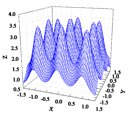
In the nonlinear function optimization, most of the optimization calculation are seeking maximum or minimum values. For example, finding the maximum value of the following nonlinear functions.
$f(x)=\frac{\sin \sqrt{x^{2}+y^{2}}}{\sqrt{x^{2}+y^{2}}}+e^{\frac{\cos 2 \pi x+\cos 2 \pi y}{2}}$ (8)
From the function simulation in figure 2, we can see that there are a lot of local maximum points for the function, the extremum position is (0, 0), its maximum value is obtained near the point.
Here, the population size is 20, the number of evolutionary is 300. In order to improve the effectiveness of the algorithm and avoid local optimal results interference, the algorithm runs 100 times, and then the average value of their results as the final results. In the algorithm, different linear decreasing inertia weight methods are adopted. And $\omega_{0}(k)$ weight method is set to a fixed weight value, that is $\omega_{\text {start}}$=$\omega_{e n d}$=1, to compare with other variable weight methods. $\omega_{\text {start}}$ is 0.9, $\omega_{e n d}$ is 0.4 and c is 10 in other variable weight methods.
Figure 2. Nonlinear function simulation
As can be seen from the table 1 and figure 3, when the inertia weight is a constant, the PSO algorithm has the fast convergence rate, but it is easy to get into local optimum and the accuracy is low; and the other variable weight PSO algorithms converge slightly slowly in the initial stage of the algorithm, but they will be strong in the latter search. In this way, it is advantageous to get the global optimal solution by jumping out of the local optimal solution, so as to improve the accuracy of the algorithm [14,15].
Figure 3. The convergence curves of mean value based on 5 different types of weights
Table 1. The algorithm performance comparison based on five kinds of inertia weight
|
$\omega$ |
Optimum solution obtained |
Average value |
The number of trapping in local optimal solution |
The number of globe optimal solution |
|
$\omega_{0}$ |
3.693 2 |
3.685 2 |
25 |
75 |
|
$\omega_{1}$ |
3.693 2 |
3.675 7 |
18 |
82 |
|
$\omega_{2}$ |
3.693 2 |
3.693 2 |
0 |
100 |
|
$\omega_{3}$ |
3.693 2 |
3.685 5 |
11 |
89 |
|
$\omega_{4}$ |
3.693 2 |
3.671 1 |
27 |
73 |
3.1 SVM regression model
The SVM regression method is different from multivariate regression analysis method, whose constructors including nonobject parameters to be eliminated needn't be established, can get theoretical optimal solution using convex quadratic optimization problem transformation through estimation and prediction of the small samples on the basis of VC dimension theory coming from statistic learning theory and structural risk minimization [16]. Sampling group points $\left\{\left(\boldsymbol{x}_{i}, y_{i}\right)\right\}_{i=1}^{N^{+}}$ in input analytical space X can be mapped to become training group points $\left(\varphi\left(x_{i}\right), y_{i}\right)$ in high dimensional Hilbert space F by SVM kernel function algorithm, and the training set $D=\left\{\left(\boldsymbol{\varphi}\left(\boldsymbol{x}_{i}\right), y_{i}\right)\right\}_{i=1}^{N^{*}}$ which have been mapped is regressed by constructing linear discriminant function in Hilbert space F. Thus the regression inverse model has better generalization ability, and the dimension disaster is avoided, which means that algorithm complexity is unrelated to sample dimension [17].
Set sample set to $\left\{\left(\boldsymbol{x}_{i}, y_{i}\right)\right\}_{i=1}^{N^{t}}$, where $\boldsymbol{x}_{i} \in \boldsymbol{R}^{d}$ is input vector, $y_{i}$ is corresponding expected value. A dual problem model constrained convex quadratic optimization is defined as
$\arg \max _{a} \omega(\alpha)=\sum_{i=1}^{N} \alpha_{i}-\frac{1}{2} \sum_{i=1}^{N} \sum_{j=1}^{N} y_{i} y_{j} \alpha_{i} \alpha_{j} K\left(\boldsymbol{x}_{i}, \boldsymbol{x}_{j}\right)$
s.t. $\sum_{i=1}^{N} \alpha_{i} y_{i}=0 ; 0 \leq \alpha_{i} \leq C, i=1,2, \cdots, N$ (9)
$\alpha_{i}$ is the Largrang multiplier and $K\left(\boldsymbol{x}_{i}, \boldsymbol{x}_{j}\right)$ is the kernel function.
Let $\boldsymbol{\alpha}^{*}=\left(\alpha_{1}^{*}, \alpha_{2}^{*}, \cdots, \alpha_{N^{+}}^{*}\right)$ be the solution vector of (9), in which usually only part of solutions are not zero. $\boldsymbol{x}_{i}$ is the input sample of corresponding nonzero solutions and serves as support vectors, which determined decision boundary. The data regression based on SVM is done to establish the fitting relationships between input x and output y, that is
$y(\boldsymbol{x})=\overline{\boldsymbol{\omega}}^{T} \boldsymbol{x}+b=\sum_{i=1}^{s} \alpha_{i} K\left(\boldsymbol{x}, \boldsymbol{x}_{i}\right)+b$ (10)
In (10), $x_{i}$ is the support vector; s is the number of the support vectors; b is the SVM offset; $\bar{\omega}$ is the weight coefficient whose number is similar to support vectors number. Gaussian radial basis function which meets Mercer condition is chosen as kernel function [18]. That is
$K\left(\boldsymbol{x}, \boldsymbol{x}_{i}\right)=\exp \left(-\frac{\left\|\boldsymbol{x}-\boldsymbol{x}_{i}\right\|}{2 \sigma^{2}}\right)$ (11)
σ is the kernel function parameter. The forecast accuracy of SVM would be improved by regulating σ properly.
3.2 Preparation of the data samples
The number of the overall sample pairs $\left(\boldsymbol{x}_{i}, y_{i}\right)$ $(i=1,2, \cdots, N)$ is $N=N_{p}+N_{t}$ and $N_{p}$ is the number of training samples ($N_{p}$ accounted for 1/2~2/3 of the overall sample number $N$), $N_{t}$ is the number of testing samples. The $N_{p}=26$ training samples and $N_{t}=25$ testing samples are randomly selected from liquid ammonia density temperature relation table (-20℃~30℃) [11].
The relation data of liquid ammonia density temperature is shown in table 2.
Table 2. Liquid ammonia density temperature relation table
|
NO. |
Temperature |
Density |
NO. |
Temperature Density |
|
|---|---|---|---|---|---|
|
℃ |
$k g / m^{3}$ |
℃ |
$k g / m^{3}$ |
||
|
1 |
-20 |
665.005 |
27 |
6 |
630.293 |
|
2 |
-19 |
663.721 |
28 |
7 |
628.897 |
|
3 |
-18 |
662.433 |
29 |
8 |
627.496 |
|
4 |
-17 |
661.141 |
30 |
9 |
626.089 |
|
5 |
-16 |
659.846 |
31 |
10 |
624.678 |
|
6 |
-15 |
658.546 |
32 |
11 |
623.261 |
|
7 |
-14 |
657.243 |
33 |
12 |
621.838 |
|
8 |
-13 |
655.936 |
34 |
13 |
620.411 |
|
9 |
-12 |
654.625 |
35 |
14 |
618.978 |
|
10 |
-11 |
653.31 |
36 |
15 |
617.539 |
|
11 |
-10 |
651.991 |
37 |
16 |
616.094 |
|
12 |
-9 |
650.668 |
38 |
17 |
614.644 |
|
13 |
-8 |
649.341 |
39 |
18 |
613.188 |
|
14 |
-7 |
648.009 |
40 |
19 |
611.726 |
|
15 |
-6 |
646.673 |
41 |
20 |
610.258 |
|
16 |
-5 |
645.333 |
42 |
21 |
608.784 |
|
17 |
-4 |
643.989 |
43 |
22 |
607.303 |
|
18 |
-3 |
642.64 |
44 |
23 |
605.817 |
|
20 |
-1 |
639.929 |
45 |
24 |
604.324 |
|
21 |
0 |
638.567 |
46 |
25 |
602.824 |
|
22 |
1 |
637.2 |
47 |
26 |
601.318 |
|
23 |
2 |
635.828 |
48 |
27 |
599.805 |
|
24 |
3 |
634.451 |
49 |
28 |
598.285 |
|
25 |
4 |
633.07 |
50 |
29 |
596.759 |
|
26 |
5 |
631.684 |
51 |
30 |
595.225 |
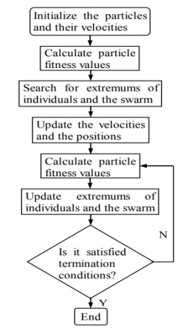
4.1 The PSO optimization algorithm design
Trained SVM with training samples is tested by MSETD which represent the standard deviation of mean square error between the density calibration values and the predicted values of testing samples, in order to reduce the dependence of parameter selection to testing samples. The experiments show these learning parameters in SVM, including boundary of Lagrange multiplier C, the condition parameter of convex quadratic optimization λ and ε-neighborhood parameter around solutions ε, have no obviously effect on the output results, but the kernel function parameter σ that have the largest influence on the output results is often difficult to identify only by trial and error [20]. Taking MSETD as fitness function, the kernel function parameter σ is optimized by virtue of PSO global search performance for optimal solutions and then the proper offset b and weight coefficient $\bar{\omega}$ are found, so that output results are optimal or suboptimal to meet the precision and accuracy of system measurement.
The fitness function can be expressed as
$f_{F}=M S E T D$ (12)
In addition, the object function is
$f_{O b j}=\min \left(f_{F}\right)=\min (M S E T D)$ (13)
The algorithm flow of PSO is shown in Figure 4.
Figure 4. The algorithm flow of PSO
4.2 The operation result of PSO
The population size of the PSO equal to 20, the maximum number of iterations is 300. Through the analysis of various inertia weight method above, and because of the nonlinearity in the selection of SVM kernel function parameter σ, the linear decreasing inertia weight ω2 is adopted here [21]. The corresponding SVM configuration parameters are set as follows: the kernel function is RBF function, regularization parameter C is 500 and the non-sensitive ε is 0.001.
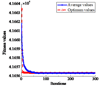
After the algorithm runs 100 times,the optimal value and the average optimal value of each iteration are obtained respectively [15, 22]. Can be seen from Figure 5, their convergence curves finally tend to be consistent. The average optimal value of each iteration in the process of optimization of the kernel function parameter σ is shown in Figure 6.
Figure 5. The convergence curves of the optimal values and the average optimal values
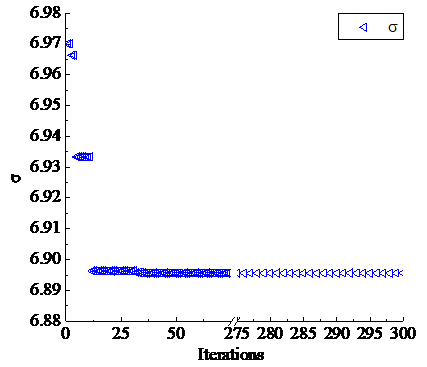
Figure 6. The average optimal value of each iteration in the process of optimization of the kernel function parameter σ
According to the results of PSO operation, MSETD, namely the standard deviation of mean square error between the density calibration values and the predicted values of testing samples, is 41656.2148 when kernel function parameter σ obtained by PSO equals 6.8956.
With the traditional quadratic expression method, the model is as follow [3]:
$\rho=\rho_{d}\left[1+\mu_{1}\left(t-t_{d}\right) \times 10^{-2}+\mu_{2}\left(t-t_{d}\right)^{2} \times 10^{-6}\right]$ (14)
Here, t [℃] is the temperature of liquid ammonia; $t_{d}$ [℃] is the reference temperature of liquid ammonia; $\rho_{d}$ [$k g / m^{3}$] is the density of liquid ammonia that correspond to$t_{d}$; $\mu_{1}$ [$10^{-2} c$] is the linear compensation coefficient of liquid ammonia; $\mu_{2}$ [$10^{-6} C^{-2}$] is the quadratic compensation coefficient of liquid ammonia.
When $t_{d}=5^{\circ} \mathrm{C}$ , then $\rho_{d}=631.684 \mathrm{kg} / \mathrm{m}^{3}$, the two endpoint temperature values -20℃and 30℃, and the density data are substituted in (14) using binary equation groups to obtain $\mu_{1}=-0.2209$ and $\mu_{2}=-3.9741$, and the relation between the temperature t and the density ρ can be established so long as $\mu_{1}$ and $\mu_{2}$ are substituted in (14) again.
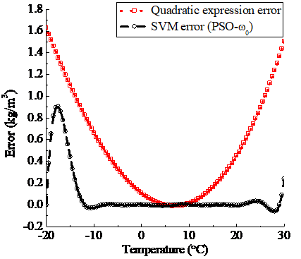
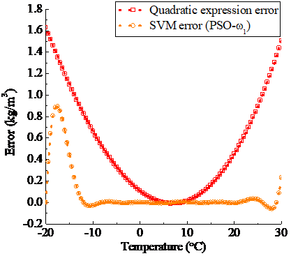
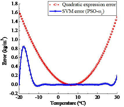
In the optimization of SVM kernel function parameter by 5 types of inertia weight PSO methods, when the inertia weights are from ω0 to ω4, the optimization results of the corresponding kernel function parameter respectively are 6.6887, 6.7576, 6.8956, 6.9921 and 7.0127. The temperature compensation of SVM regression is carried out by respectively using these kernel function parameter values, the comparison results of their error curves and the error curve of the conventional quadratic expression method are shown in (a)~(e) of Figure 7.
a) Weight is ω0
b) Weight is ω1
c) Weight is ω2
d) Weight is ω3
e) Weight is ω4
Figure 7. The error contrast of quadratic expression method and SVM (optimized by PSO when weights are ω0, ω1, ω2, ω3 and ω4 respectively) method
The error contrast effect of SVM temperature compensation optimized by 5 types of inertia weight PSO methods is shown in Figure 8.
Figure 8. The error contrast of SVM (optimized by PSO based on 5 different types of weights) method
The temperature compensation accuracy of the SVM method based on the variable weight PSO is significantly higher than that of the traditional quadratic expression method, and the optimization effect of PSO using the linear decreasing inertia weight ω2 is better than others.
Based on experiment data processing and theoretical analysis, the main results obtained in this study can be summarized as follows:
(1) SVM regression method can play an important role in temperature compensation only if the corresponding parameters such as kernel function parameter σ are well configured.
(2) The temperature compensation accuracy of the SVM method based on the variable weight PSO is significantly higher than that of the traditional quadratic expression method, and the selection of weight method has the effect on the optimization effect. Therefore, it’s important to find the appropriate weight method by comparison to improve the effect of PSO in the SVM parameter optimization.
(3) Using the quadratic expression method or SVM regression method for temperature compensation, the temperature compensation effect is the best in the middle of the temperature region, but that of the two ends of the region is relatively poor. Therefore, in the application, pay attention to the choice of reasonable temperature region or adopt other assistant compensation way [23].
By using SVM regression temperature compensation method based on variable weight PSO, the measurement accuracy and the environmental adaptability of volumetric flowmeter can be significantly improved in the measurement of liquid ammonia quality, the method will have the wide application prospects in modern coal chemical industry.
Science Foundation of China under the contract number 61305147 and the Natural Science Foundation of Chongqing under the contract number cstc2012jjA10129.
1. A. Orooji and S. Hosseininia, The rupture of a liquid ammonia storage tank study, Ammonia Plant Safety and Related Facilities, vol. 55, pp. 187-205, 2014.
2. A. Kumagi and T. Toriumi, Pressure-volume-temperature relationship of liquid ammonia, Journal of Chemical and Engineering Data, vol. 16(3), pp. 293-295, 1971.
3. G. Ji, The flow measurement instrument application skills. Beijing: Chemical Industry Press, Beijing, 2012.
4. H. Yurtseven and H. Karacali, Temperature and pressure dependence of molar volume in solid phases of ammonia near the melting point, Journal of Molecular Liquids, vol. 142(1-3), pp. 88-94, 2008.
5. L. CH. Xing, Y. F. Geng, CH. Q. Hua, H. Hao and A. Rieder, A combination method for metering gas-liquid two-phase flows of low liquid loading applying ultrasonic and Coriolis flowmeters, Flow Measurement and Instrumentation, vol. 37, pp. 135-143, 2014.
6. N. Mathies, methods for the validation of liquid flow measuring systems, Euroheat and Power (English Edition), vol. 11(4), pp. 54-57, 2014.
7. S. Yoon, D. E. Macphee and M. S. Imbabi, Estimation of the thermal properties of hardened cement paste on the basis of guarded heat flow meter measurements, Thermochimica Acta, vol. 588, pp. 1-10, 2014.
8. J. B. Yu, J. Li, Q. L. Dai, D. Li, X. B. Ma and Y. P. Lv, Temperature compensation and data fusion based on a multifunctional gas detector, IEEE Transactions on Instrumentation and Measurement, vol. 64(1), pp. 204-211, 2015.
9. H. N. Zhang and Y. H. Ren, Frequency processing and temperature-pressure compensation of the vortex flowmeter based on two-phase flow, International Journal on Smart Sensing and Intelligent Systems, vol. 7(3), pp. 1326-1346, 2014.
10. J. Ch. Cheng, J. Ch. Fang, W. R. Wu and J. L. Li, Temperature drift modeling and compensation of RLG based on PSO tuning SVM, Measurement: Journal of the International Measurement Confederation, vol. 55, pp. 246-254, 2014.
11. F. M. Gao and T. Lin, Application of SVM optimization based on GA in electronic sphygmomanometer data fusion. International Journal of Computer Science Issues, vol. 10(1-1), pp. 1-6. 2013.
12. A. Arulmozhi and M. Ezhilarasi, Maximal information compression index (Mici) and PSO based detection of jaundice, Journal of Multiple-Valued Logic and Soft Computing, vol. 24(5-6), pp. 583-597, 2015.
13. P. J. García Nieto, E. García-Gonzalo, F. Sánchez Lasheras and F.J. De Cos Juez, Hybrid PSO-SVM-based method for forecasting of the remaining useful life for aircraft engines and evaluation of its reliability, Reliability Engineering and System Safety, vol. 138, pp. 219-231, 2015.
14. L. Ni, J. C. Jiang and Y. Pan, Leak location of pipelines based on transient model and PSO-SVM, Journal of Loss Prevention in the Process Industries, vol. 26(6), pp. 1085-1093, 2013.
15. P. J. García Nieto, E. García-Gonzalo, J. R. Alonso Fernández and C. Díaz Muñiz, Hybrid PSO-SVM-based method for long-term forecasting of turbidity in the Nalón river basin: A case study in Northern Spain, Ecological Engineering, vol. 73, pp. 192-200, 2014.
16. J. Bin and G. Zhi, WeiThe fault diagnosis of wind turbine gearbox based on QGA-LSSVM, Applied Mechanics and Materials, vol. 543-547, pp. 950-955, 2014.
17. S. L. Zhou, J. Liao and X. J. Shi, SVM parameters selection method based on Fisher criterion and maximum entropy principle, Control and Decision, vol. 29(11), pp. 1991-1996, 2014.
18. P. Wu and T. Lin, Research on identification modeling of sheathed thermocouple sensor based on hybrid QGA-SVM, Chinese Journal of Scientific Instrument, vol. 35(2), pp. 343-349, 2014.
19. Ch. Sudheer, N. Anand, B. K. Panigrahi and Sh. Mathur, Streamflow forecasting by SVM with quantum behaved particle swarm optimization, Neurocomputing, vol. 101, pp. 18-23, 2013.
20. A. S. M. Murugavel and S. Ramakrishnan, Optimal feature selection using PSO with SVM for epileptic EEG classification, International Journal of Biomedical Engineering and Technology, vol. 16(4), pp, 343-358, 2014.
21. H. H. Tsai, Y. Sh. Lai and Sh. Ch. Lo, A zero-watermark scheme with geometrical invariants using SVM and PSO against geometrical attacks for image protection, Journal of Systems and Software, vol. 86(2), pp. 335-348, 2013.
22. K. V. Santhosh and B. K. Roy, Support vector machine based adaptive calibration technique for resistance temperature detector, IFAC Proceedings Volumes (IFAC-Papers Online), vol. 3, pp. 546-551, 2014.
23. P. Ligza, Advanced temperature compensation and correction techniques in thermal anemometry, Instrumentation Science and Technology, vol 43(1), pp. 21-43, 2015.