OPEN ACCESS
Lithography manufacturing process of linear grating is a complex precision manufacturing process, good environmental conditions are conducive to improve product quality, air velocity and temperature field formed by the air conditioning of a certain lithography workshop are simulated by the CFD in this paper and the parameters of the air conditioning is determined to meet the technology requirement, while influence of air temperature and velocity to the air flow of workshop is researched. The thermal deformation accounts for comprehensive deformation of 0.89%. The proportion is a great impact in precision manufacturing and need to be fully considered in the subsequent equipment improvements.The research can provide a theoretical basis for the actual production, test cost and test time can be reduced.
Lithography, CFD, Velocity field, Temperature field.
Linear grating is a kind of feedback device which works based on the optical principle of grating, it's the key core components of equipment manufacturing in China. The traditional grating preparation methods include mechanical scribing, film replication and so on. However, the diversification of form and functional of grating put forward higher requirements for the preparation technology. Currently widely used is photolithography[1][2]. Lithography process is a complex precision manufacturing process, many factors directly affect the manufacturing precision of grating ruler. A good processing environment can improve the quality of grating ruler to a certain extent[3]. So it is hoped that in the planning and design stage will be able to learn more about air velocity field, temperature field, etc. which formed by the air-conditioning and ventilation and make a reasonable air conditioning parameters and space layout. In civil and industrial buildings air conditioning thermostat works, rational organization of air flow within the air-conditioned room has become a very important issue.
Treated by the air conditioning system, air flow from the air supply inlet into the air-conditioned rooms, and then discharge from the return air after the heat transfer with indoor air, which would inevitably lead to the formation of some form of air flow patterns and velocity field of the
indoor air flow. Velocity field is often considered as the basis and premise of the temperature field, humidity field and concentration field, so air-conditioned rooms with different requirements, often require different forms of air flow patterns and velocity field. Airflow design task is to rationally organize air temperature, flow rate and humidity parameters of indoor air flow to meet the comfort air conditioning design requirements of people or manufacturability workshop air conditioning design requirements. Reasonable flow in room or not, not only directly affect the success of the air conditioning, but also have an impact on energy-saving effect of the entire air-conditioning system.
Many factors affect the airflow, such as the type, number and location of air inlet., the location of the outlet, air parameters (such as air temperature, outlet velocity, etc.), the geometry size of air conditioning room and a variety of heat, pollution and other disturbances. Air velocity and temperature field formed by the air conditioning of a certain lithography workshop are simulated by the CFD in this paper. The velocity field and temperature field in different conditions are reproduced by numerical simulation which not only intuitive and beneficial scheme comparison, but also saves a lot of manpower, material resources, greatly shorten the design cycle. It is of great significance to improve indoor air quality, improve the level of control pollutants of indoor air and ensure the realization of optimal design.
CFD (Computational Fluid Dynamics) equals to a virtual experiment in computer which used to simulate the actual fluid flow situation. The basic principle is the numerical solution of differential equations of fluid flow control. The discrete distribution of fluid flow in a continuous area can be got and thereby approximate simulation of fluid flow. Almost all flow phenomena from laminar flow to turbulent, flow steady to unsteady, incompressible to compressible, non-sticky to sticky etc. can be analyzed. The FLUENT software is used in this article.
The basic theories of CFD similar to fluid mechanics theory, mass conservation equation, momentum conservation equation and energy conservation equation is the foundation and core of CFD theory. First, the mathematical model of research questions is established, the general differential equations for viscous fluid flow is as Equation (1):
$\frac{\partial}{\partial t}(\rho \Phi)+\nabla \cdot(\rho \vec{U} \Phi)=\nabla \cdot\left(\Gamma_{\Phi} \operatorname{grad} \Phi\right)+S_{\Phi}$ (1)
Where, $\Phi$ —universal variable, $\rho$ —generalized density, U—velocity vector, $\Gamma_{\Phi}$ —generalized diffusion coefficient, $\mathrm{S}_{\Phi}$ —generalized source term.
The method to solve the practical problem is a discrete area. Differential equation becomes algebraic equations after discretization. The form is as Equation (2):
$a_{p} \Phi_{p}=a_{E} \Phi_{E}+a_{W} \Phi_{W}+a_{N} \Phi_{N}+a_{S} \Phi_{S}+a_{T} \Phi_{T}+a_{B} \Phi_{B}+b$ (2)
Where, a—discrete equation coefficients,Φ—variable value of each grid node, b—the source term of discrete equation, index indicates the basic grid and adjacent six nodes, respectively. Discrete distribution of the flow field can be obtained by numerical calculation to realize simulation of current situation[4][5].
Many previous test results show that the buoyancy amendments three-dimensional k-ε turbulence model equations is superior to other models, make the following assumptions are made to simplify the calculations.
(1) The air flow is turbulent flow;
(2) Consider the indoor air as incompressible fluid, and in accordance with Boussniosq assumption that that the fluid density changes only affect buoyancy;
(3) The indoor gas belongs to Newtonian fluid, as steady flows;
(4) Assuming that the flow field with high turbulence Re, isotropic turbulent viscous fluid;
(5) Ignore the Energy dissipation of the energy equation due to cohesive role;
(6) Does not consider the impact of air infiltration, which means a good air tightness of the simulated room.
Based on the above assumptions, the differential equation of air flow and heat transfer mathematical model in air conditioning room are as follows:
Continuity equation is as Equation (3):
$\frac{\partial\left(\rho \mathrm{u}_{\mathrm{i}}\right)}{\partial \mathrm{x}_{\mathrm{i}}}=0$ (3)
The momentum equation is as Equation (4):
$\begin{aligned} \frac{\partial(\rho \mathbf{u_{i}} \mathbf{y_{i}})}{\partial \mathbf{x}_{\mathbf{i}}}=&-\frac{\partial}{\partial \mathbf{x}_{\mathbf{j}}}\left(\mathbf{P}+\frac{2}{3} \rho \mathbf{k}\right)+\frac{\partial}{\partial \mathbf{x}_{\mathbf{i}}}\left[\left(\mu+\mu_{\mathbf{j}}\right)\left(\frac{\partial \mathbf{u}_{\mathbf{i}}}{\partial \mathbf{x}_{\mathbf{j}}}+\frac{\partial \mathbf{u}_{\mathbf{j}}}{\partial \mathbf{x}_{\mathbf{j}}}\right)\right]+\mathbf{g}_{\mathbf{i}}\left(\rho_{\mathrm{ref}}-\rho\right) \end{aligned}$ (4)
Energy equation is as Equation (5):
$\frac{\partial\left(\rho u_{i} h\right)}{\partial x_{i}}=\frac{\partial}{\partial x_{i}}\left[\left(\frac{\mu}{p_{r}}+\frac{\mu_{t}}{\sigma_{t}}\right) \frac{\partial h}{\partial x_{i}}\right]+q$ (5)
Turbulent energy equation(k equation) is as Equation (6):
$\begin{aligned} \frac{\partial\left(\rho u_{i} k\right)}{\partial x_{i}}=\frac{\partial}{\partial x_{i}} &\left[\left(\mu+\frac{\mu_{t}}{\sigma_{k}}\right) \frac{\partial k}{\partial x_{i}}\right]+ \mu_{t} \frac{\partial u_{i}}{\partial x_{j}}\left(\frac{\partial u_{i}}{\partial x_{j}}+\frac{\partial u_{j}}{\partial x_{i}}\right)-\rho \epsilon+G \end{aligned}$ (6)
Turbulent energy dissipation equation($\varepsilon$ equatio) is as Equation (7):
$\frac{\partial\left(\rho \mathrm{u}_{\mathrm{i}} \varepsilon\right)}{\partial \mathrm{x}_{\mathrm{i}}}=\frac{\partial}{\partial \mathrm{x}_{\mathrm{i}}}\left[\left(\mu+\frac{\mu_{\mathrm{t}}}{\sigma_{\varepsilon}}\right) \frac{\partial \varepsilon}{\partial \mathrm{x}_{\mathrm{i}}}\right]+\frac{\varepsilon}{\mathrm{k}} \mathrm{c}_{1} \mu_{\mathrm{t}} \frac{\partial \mathrm{u}_{\mathrm{i}}}{\partial \mathrm{x}_{\mathrm{j}}}\left(\frac{\partial \mathrm{u}_{\mathrm{i}}}{\partial \mathrm{x}_{\mathrm{j}}}+\frac{\partial \mathrm{u}_{\mathrm{j}}}{\partial \mathrm{x}_{\mathrm{i}}}\right)-\mathrm{c}_{2} \rho \frac{\varepsilon^{2}}{\mathrm{k}}+\mathrm{c}_{3} \mathrm{G}_{\mathrm{k}}^{\varepsilon}$ (7)
Here G for the buoyancy, Produced by temperature difference effect is as Equation (8):
$G=g_{i} \beta \frac{\mu_{t}}{\sigma_{t}} \frac{\partial T}{\partial x_{i}}$ (8)
$\mu_{t}$ For the turbulent viscosity coefficient is as Equation (9):
$\mu_{t}=\frac{C_{u} \rho K^{2}}{\varepsilon}$ (9)
$\mathrm{u}_{\mathrm{i}}-$ The $\mathrm{x}_{\mathrm{i}}$ direction of the time - averaged velocity
$\mathrm{u}_{\mathrm{j}}-$ The $\mathrm{x}_{\mathrm{j}}$ direction of the time - averaged velocity
$\rho_{\text {ref }}-$ For the reference density
$\rho$ —Air density, kg/m3;
P—Air static pressure, Pa;
$\mu$ —Air laminar viscosity coefficient, Pa·s;
$\mu_{t}$ —Air turbulence viscosity coefficient, Pa·s;
T—The air temperature, ℃;
gj For j in the direction of acceleration;
h—Air enthalpy ,J/kg;
q—Heat yield, W;
$\beta$ Volume expansion coefficient, K-1;
$\mathrm{P}_{\mathrm{r}}$ —Turbulent prandtl number;
c and $\sigma$ —Empirical coefficient
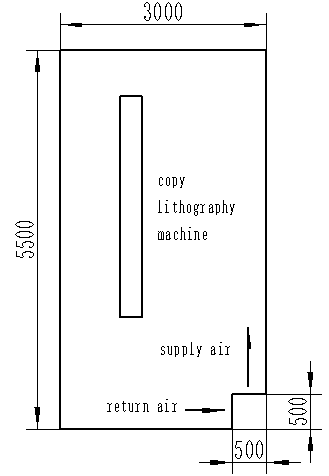
The research object of this topic is the air distribution of a standard grating ruler lithography workshop. Workshop simplified physical model as shown in Figure 1.The whole workshop is a rectangular area of 3 m x 5.5 m, the bottom right corner of the workshop is equipped with air conditioning, the supply and return air direction as shown in Figure 1. Copy lithography machine is placed in the workshop. In accordance with the technical requirements, considering the precision and investment economy, the temperature of the grating ruler manufacturing environment should be controlled at 20 ± 0.5 ℃.
The actual lithography workshop is simplified to a two-dimensional model by the ICEM-CFD in this paper, and then the grid is introduced into FLUENT. The grid has no negative volumes to meet the computing needs after inspection. The grid model as shown in Figure 2.
Figure 1. Workshop physical model
Figure 2.Workshop grid model
The CFD model can be established in FLUENT. The single precision solver based on pressure should be chosen. The Standard k-ε model of turbulence model should be selected, this model is used more often , the amount of calculation is moderate, it has more data accumulation and relatively high accuracy. The simulation effect is not good enough for the complex flow with larger curvature and stronger pressure gradient. This model is used for general engineering calculation, because of its convergence and
accuracy also can meet the computing requirements. The standard wall function method is selected for its more applications, small computational amount and high accuracy. It is suitable for high Reynolds number flow. Energy equation needs to be activated due to the heat transfer. Material Properties keep the default of air properties. Boundary conditions of the import, the export and the wall are defined[6][7], as shown in Table 1.
Table 1. The boundary conditions of grating ruler lithography workshop
|
Zone name |
Type |
Velocity(m/s) |
Turbulence Intensity(%) |
Hydraulic Diameter(m) |
Temperature(K) |
|
In |
velocity-inlet |
1 |
0.5 |
0.5 |
293 |
|
Out |
pressure-outlet |
/ |
0.5 |
0.5 |
298 |
|
Wall |
wall |
/ |
/ |
/ |
298 |
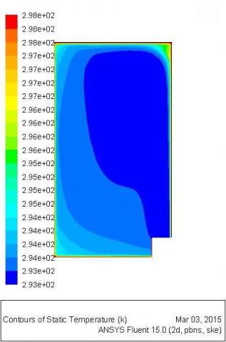
The above CFD model will be submitted into analysis and calculation, and then enters the post-processing. The airflow velocity and the temperature of the workshop are shown in Figure 3 and Figure 4, respectively.
Figure 3. Velocity nephogram
Figure 4. Temperature nephogram
To further quantitative research the air case near the guide rail of the copy lithography machine worktable , a long straight line of 3m is created in the area , then the data on this line is extracted and drawn on a graph. Velocity curve shown in Figure 5 shows, the airflow velocity of the region is fluctuated within the range of 0.34m / s-0.39m / s. Temperature curve shown in Figure 6 shows, the temperature of the region is fluctuated within the range of 20.12℃—20.29℃,which meets the environmental requirements of the lithography workshop.
Figure 5. The airflow velocity curve near the guide rail of the copy lithography machine worktable
Figure 6. The airflow temperature curve near the guide rail of the copy lithography machine worktable
It is emphasized that the lithography environments of different specifications are different in actual production. The air conditioning parameters can be determined by means of CFD method to improve product quality, shorten test time and cost as well. Therefore, the guide rail midpoint (coordinate(1.2,3.2)) of the copy lithography machine worktable is seen as a fixed reference point in this paper. Research the impact of the supply air temperature and velocity on the node of the airflow provides a theoretical basis for the actual production. The analysis process is same with the aforementioned[8].
Keeping the other boundary conditions remain unchanged, the calculation is submitted after only changing the supply air temperature. The calculation results are shown in Table 2,and the draw curve is shown in Figure 7.
Table 2. Effect of supply air temperature on the air distribution
|
supply air temperature(℃) |
Node airflow temperature(℃) |
Node airflow velocity(m/s) |
The rate of change of node airflow temperature |
|
20 |
20.19992 |
0.39142662 |
/ |
|
21 |
21.16119 |
0.39142662 |
4.76% |
|
22 |
22.12079 |
0.39142662 |
4.53% |
|
23 |
23.08069 |
0.39142662 |
4.34% |
|
24 |
24.04025 |
0.39142662 |
4.16% |
|
25 |
24.99957 |
0.39142662 |
3.99% |
Figure 7. Effect of supply air temperature on the air distribution
This shows the airflow temperature at the node is rose accordingly when the supply air temperature for each additional 1℃, The temperature change rate is about 4%. And the airflow velocity at the node is not affected.
Keeping the other boundary conditions remain unchanged, the calculation is submitted after only changing the supply air velocity. The calculation results are shown in Table 3,and the draw curve is shown in Figure 8.
Table 3. Effect of supply air velocity on the air distribution
|
supply air velocity(m/s) |
Node airflow temperature(℃) |
Node airflow velocity(m/s) |
The rate of change of node airflow velocity |
|
1.0 |
20.19992 |
0.39142662 |
/ |
|
1.1 |
20.17792 |
0.38597089 |
-1.39% |
|
1.2 |
20.14954 |
0.4560509 |
18.16% |
|
1.3 |
20.20889 |
0.48396611 |
6.12% |
|
1.4 |
20.11737 |
0.30418363 |
-37.15% |
|
1.5 |
20.18686 |
0.60057342 |
97.44% |
|
1.6 |
20.18356 |
0.54710001 |
-8.90% |
|
1.7 |
20.18549 |
0.69867462 |
27.71% |
|
1.8 |
20.11008 |
0.38709339 |
-44.60% |
|
1.9 |
20.19937 |
0.67249489 |
73.73% |
|
2.0 |
20.11765 |
0.78637576 |
16.93% |
Figure 8. Effect of supply air velocity on the air distribution
This shows effect of changes in supply air velocity on node airflow temperature is not obvious, the temperature is maintained at about 20 ℃. The node airflow velocity is wavy changing when the supply air velocity is raising. But overall tends to increase.
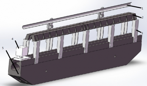
Based on the above analysis of airflow, it is necessary to further study the integrated deformation situation of the long grating lithography. The existing measuring precision lithography copy machine is mainly composed of base, long grating placed stents and so on. The three-dimensional model established with SolidWorks software is shown in Figure 9 which 1is the gland in institutions, 2 for stent for processing, 3, 4 for the light, 5 for the base.
Figure 9. The 3D model
When lithography copying machine works, it not only affected by the action of static force, dynamic force, but also affected by the surrounding environment, so it is important to the to improve the accuracy of the lithographic copy by research surrounding environment.
In this paper, using ABAQUS is used to research the deformation of lithography copying machine. To reduce the computational cost in ensuring the accuracy of the premise, the original 3 d model need to be properly simplified, such as remove the structure in this model the smaller of thin face, chamfer, etc.
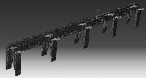
The simplified assembly model is introduced into ABAQUS software, the definition of processing base material HT250, a density of 7280kg / m3, the elastic modulus of 1.38x10⁵MPa, Poisson's ratio of 0.156, defined as 45 steel scaffold, a density of 7890kg / m3, elastic modulus 2.09x10⁵MPa, Poisson's ratio of 0.269. According to the actual work situation, the interaction between the various parts of the contact surfaces are applied . The finite element model is shown in Figure10.
Figure10. The finite element model
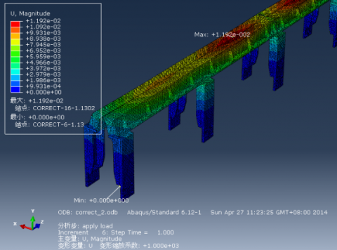
By defining the material density and weight of each parts gravity acceleration added automatically. Applying a heat load refer to Figure 4.4, After submitting analysis and calculation, the processing seat integrated deformation as shown in Figure11. The maximum displacement is 1.192e-002mm, in which the direction of gravity displacement is 5.925e-003mm.
Figure11. The integrated displacement nephogram
If you simply consider the thermal deformation after heat load is applied with reference to Figure 4.4 to calculate the temperature profile and submit, the processing base thermal deformation as shown in Figure12.
Figure12. The thermal displacement nephogram
From the analysis results, the maximum displacement amplitude generated by the thermal deformation is 1.067e-004mm. That distortion accounts for comprehensive deformation of 0.89%. The proportion is a great impact in precision manufacturing and need to be fully considered in the subsequent equipment improvements.
Good lithographic environment will help improve the quality of the long grating copy lithography. The air distribution situation of a specification long grating lithography workshop is analysis by CFD in this paper. The results show, they can meet the environment requires of a long grating copy lithography process when the air supply temperature is 20℃and the air supply velocity is 1m/s. Meanwhile, the effect of changes in supply air temperature and supply air velocity on the workshop air distribution is also researched in this paper. When the supply air temperature for each additional 1℃,the airflow temperature of the reference node is increase of about 4% accordingly ,but the air flow velocity has little effect. With the increase of supply air velocity, the node airflow velocity is overall wavy changing, air flow temperature changed little. On this basis, the paper further application a heat load on the rails of lithography copy machine, the analysis results show that the thermal deformation accounts for comprehensive deformation of 0.89%. The proportion is a great impact in precision manufacturing and need to be fully considered in the subsequent equipment improvements.
The analysis results of this paper provide a theoretical basis for the actual production. The research method has a certain guiding significance for the rational organization of airflow within the air-conditioned room.
The project is supported by Guizhou Science and Technology Department (No. (2012) 6020 and No.(2013) 6003).
1. TANG Tianjin, CAO Xiangqun and LIN Bin. The summary of manufacturing metrology grating[J]. Optical Instrument, 26(4): 62-67, 2004.
2. BAI Shan. Lithography exposure technology evolution[J]. Integrated Circuit, (12): 3-6, 2003.
3. DONG Huijun. Effect of temperature on the duplicate grating diffraction wave front[J]. Instruments and analysis monitoring, (2): 31-34, 2000.
4. XUE Dianhua. Air conditioning[M].Beijing: Tsinghua University Press, 1998.
5. TAO Wencuo. Computational fluid dynamics and heat transfer[M]. Beijing: China Building Industry Press, 1991.
6. ZHAO Qin, WANG Jing. Fluent software application in the field of hvac[J]. Refrigeration and Air Conditioning, (1): 15-18, 2003.
7. TAN Hongwei. Computational fluid dynamics appli-cations in construction environmental engineering[J]. Heating Ventilation Air Conditioning, (4): 31-36, 1994.
8. ZHAO Bin,LI Xianting, YAN Qisen. Using CFD method to improved the design of indoor non-isothermal supply airflow distribution[J]. Application foundation and Engineering Sciences journal, 12(4): 376-386, 2002.
9. Esper A, Muhlbauer W. Solar tunnel dryers for fruits[J]. Plant Research and Development, 1996, 44: 61-80.
10. Lee D S, Pyuh Y R. Optimization of operating conditions in tunnel drying of food[J]. Drying Technology, 1993, 11(5): 1025-1052.
11. Hossain M A, Bala B K. Drying of hot chilli using solar tunnel drier[J]. Solar Energy, 2007, 81(1): 85-92.
12. Sacilik K, Keskin R, Elicin A K. Mathematical modeling of solar tunnel drying of thin layer organic tomato[J]. Journal of Food Engineering, 2006, 73(3): 231-238.
13. Mabrouk S B, Khiari B, Sassi M. Modeling of heat and mass transfer in a tunnel dryer[J]. Applied Thermal Engineering, 2006, 26(17/18): 2110-2118.
14. Han Qinghua, Wu Haihua, Ye Jinpeng, et al. Monitoring and controlling system of temperature and humidity for tunnel-type dryer[J]. Transactions of the Chinese Society for Agricultural Machinery, 2010, 41(4): 119-123.
15. Kittas C, Katsoulas N, Baille A. Influence of greenhouse ventilation regime on the microclimate and energy partitioning of a rose canopy during summer conditions[J]. Journal of Agricultural Engineering Research, 2001, (02): 349-360.
16. Lee I, Short T H. Two-dimensional numerical simulation of natural ventilation in a multi-span greenhouse[J]. Transactions of the American Society of Agricultural Engineers, 2000, (01):745-753.
17. Mistriosis A, Bot G P A, Picuno P, Scarascia-Mugnozza G. Analysis of the efficiency of greenhouse ventilation using computational fluid dynamics[J]. Agic For Meteorol,1997,(01):217-228.
18. Wolfstein M. The velocity and temperature distribution of one-dimensional flow with turbulence augmentation and pressure gradient[J]. Int J Heat and Mass Transfer, 1969, 12(3): 301-318.
19. Nielsen P V,Restivo A,Whitelaw J H. The velocity characteristics of ventilated rooms[J]. J Fluids Engineering, 1978, 100(3):291-298.
20. Baly D, Mergui S, Niculae C. Confined turbulent mixed convection in the presence of a horizontal buoyant wall jet[J].ASME,HeatTransferDivision,(Publication)HTD,1992,213:65-72.
21. Cheesewright R, King K J, Ziai S. Experimental data for the validation of computer codes for the prediction of two-dimensional buoyant cavity flows [J]. ASME, Heat Transfer Division,(Publication) HTD,1986,60:75-81.
22. Hinze J O. Turbulence[M]. New York:McGraw- Hill Book Company,1975.
23. A llard F, Inard C. Naturalandm ixed convection in rooms: Prediction of thermal stratification and heat transfer by zonalmodels[C ]. ISRACV, 1992, 335-342.
24. TogariS, AraiY, M iuraK. A simplified model for predicting vertical temperature distribution in a large space[A ]. ASHRAE Transactions 99(1)[C ]. 1993. 88-99.
25. Inard C, BouiaH, Dalicieux P. Prediction of air temperature distribution in buildings with a zonal model[J].Energy and Buildings, 1996, 24: 125-132.
26. Okushima L, Sase S, Nara M. A support system for natural ventilation design of greenhouses based on computational aerodynamics[J]. Acta Horticulturae, 1989, 248: 129-136.
27. Mistriotix A, Bot G P A, Picuno P, et al. Analysis of the efficiency of greenhouse ventilation with computational fluid dynamics[J]. Agricultural Forestry Meteorology, 1997, 85:317-328.
28. Kim Keesung, Yoona Jeongyeo, KwonHyuckjin, et al. 3-D CFD analysis of relative humidity distribution in greenhouse with a fog cooling system and refrigerative dehumidifers[J]: Biosystems Engineering, 2008, 100(2): 245-255.