OPEN ACCESS
To evaluate the flood risk of Black River efficiently and conveniently, the deluge gradual processing in black river gold basin reservoir is established within the one- dimension model and two-dimension model of hydrodynamic coupling. Triangular unstructured grid is adopted to accommodate height and large span, as well as complex underlying surface of Mountain Rivers. Lateral connection, time synchronization and corresponding coupling space node are applied within coupling of one- dimension model and two-dimension model. The numerical simulation of flood in Black river gold basin reservoir which is in different frequencies is in the framework of established coupling model. As a result, the water depth and distribution of flow field in different time are obtained within the calculation areas. Based on the results of coupling simulation, the flood risk map and the analysis of importance of dam break as well as the risk of flood-hit population proceeded. The results coming from the mentioned simulation could provide basis to alarm of Black River flood and evaluation of disaster loss.
flood routing, unstructured grids, coupling simulation, risk analysis, lateral connection.
Papers should be prepared according to present instructions and printed on high-quality white paper, A4 size. Papers are to be sent to the Editor or the managing editor who handled your manuscript.
Combining hydrodynamics [1] and numerical simulation [2] is a significant method of studying watercourse flood risk, referring to the calculation and analysis of deluge risk, which is the core and base portion of flood risk graph compilation. As the flood inundates the river way, two dimension is the main path to the research [3-5]. For example, X. M. Yuan [6] established two-dimension hydrodynamic model to simulate the flood inundating the river way and embankment as well as the gradual progress of flood routing in irrigated area. Meanwhile, the meshless methods, such as particle [7] and SPH [8-9], are still in the research process, resulting in the unstructured grid method [10] being chosen as the main path to establish model of two-dimension flood routing. One-dimension hydrodynamic coupling model and two- dimension hydrodynamic coupling model could simulate much faster and calculate more appropriately during the process of flood inrush [11]. Scholars within China and other nations [12-14] coupled one-dimensional saint venant equations and different two-dimensional model separately, even the three-dimensional model to calculate and simulate hydrodynamic force. The core of coupling calculation is about the fluency of mutual calculation based on coupling points from one-dimensional model and two- dimensional model. In order to ensure the calculation fluency, many scholars [15-17] have applied ‘conservation of flow quantity’, ‘overlapping calculation areas’, and ‘weir flow formula’ to couple the connection. Based on the GIS [18-20], combining flood processing model of hydraulics, the flood process within inundated area is simulated, resulting in the important data of inundated areas, water depth and time of process, as well as other significant data in flood risk analysis, comparing with the simulation process of one-dimensional model [21], three one-dimensional model [22], and coupling model [23]. As a result, the analysis model of flood risk is established [24], leading to high convenience and efficiency of analysis process within deluge risk. Besides, reliable data is produced to draw the flood risk map.
Although the flood processing model and the risk analysis research have developed in huge advance, the problems waiting to be studied are as follow:
(a) Homogeneous mesh model could not guarantee the calculation efficiency and model accuracy at the same time, when being applied to Mountain Rivers with complex underlying surface and wide areas.
(b) The core portion refers to the interaction of data, reflected by the calculation of one-dimension and two-dimension model.
According to the problems above, the report referenced the research by other scholars, established one-dimension and two-dimension coupling model, by lateral connection, as well as mesh encryption towards different underlying surfaces, simulated process of flood into reservoir in different frequency, expanding in downstream areas. As a result, the flood risk map was drawn to analyze the importance of dam bursting flood, providing data evidence towards Black River flood alarm and disaster loss evaluation.
2.1 Principle of One-dimensional Model
One-dimensional calculation model is based on the vertical integration of substance and momentum conservation equations, the application of unsteady flow Saint-Venant equations to simulate the flow of the river or estuary state.
$\left\{\begin{array}{c}\frac{\partial A}{\partial t}+\frac{\partial Q}{\partial x}=q \\ \frac{\partial Q}{\partial t}+\frac{\partial\left(\alpha \frac{Q^{2}}{A}\right)}{\partial x}+g A \frac{\partial h}{\partial x}+\frac{g Q|Q|}{C^{2} A R}=0\end{array}\right.$ (1)
In the formula: A is the cross section area, m2; t is the time point of the coordinates calculated; Q is overcurrent flows. m3/s; x is the space coordinate calculation points; q is lateral inflow of flow, m3/s; α is the momentum correction factor; h is the water level, m; g is the acceleration of gravity, m/s2; C is the Chezy coefficient; R is the hydraulic radius.
Equations using the Abbott-Ionescu six implicit finite difference scheme to solve. The discrete form at each grid point is not to calculate the flow and water levels at the same time, but according to the order of alternate calculation of flow and water level, called Q and H. Abbott-IonescuFormat with a high accuracy, good stability. After discrete linear equations by chasing method.
2.2 Principle of Two-dimensional Model
Due to the horizontal scale is much larger than the vertical scale of flood movement, depth and flow rate of the hydraulic parameters change in the vertical direction is much smaller than the change in the horizontal direction, thus the three-dimensional flow equation can be integrated along the depth, and take an average depth, resulting in a two-dimensional shallow water flow equations of motion.
Flow continuity equation:
$\frac{\partial Z}{\partial t}+\frac{\partial(h u)}{\partial x}+\frac{\partial(h v)}{\partial y}=0$ (2)
Flow equations of motion:
$\frac{\partial u}{\partial t}+\frac{\partial u^{2}}{\partial x}+\frac{\partial v u}{\partial y}=f v-g \frac{\partial \eta}{\partial x}-\frac{1}{\rho_{0}} \frac{\partial p_{a}}{\partial x}-\frac{1}{\rho_{0} h}\left(\frac{\partial s_{x x}}{\partial x}+\frac{\partial s_{x y}}{\partial y}\right) +F_{u}+u_{s} S$ (3)
$\frac{\partial v}{\partial t}+\frac{\partial v^{2}}{\partial y}+\frac{\partial u v}{\partial x}=-f u-g \frac{\partial \eta}{\partial y}-\frac{1}{\rho_{0}} \frac{\partial p_{a}}{\partial y}-\frac{1}{\rho_{0} h}\left(\frac{\partial s_{y x}}{\partial x}+\frac{\partial s_{y y}}{\partial y}\right) +F_{v}+v_{s} S$ (4)
In the formula: t is the time, s; x is the transverse spatial coordinate, m; y coordinates for vertical space, m; Z is a water level at the x, y, m; h is the water depth at the x, y, m; u is the x-direction velocity component, m/s; v is the y-direction velocity component, m/s; g is the acceleration of gravity, m/s2; nz is the Manning coefficient; fv, fu is the Coriolis acceleration term; $g \frac{\partial \eta}{\partial x}, g \frac{\partial \eta}{\partial y}$ is the Surface water level acceleration term; $\frac{1}{\rho_{O}} \frac{\partial p_{a}}{\partial x}, \frac{1}{\rho_{0}} \frac{\partial p_{a}}{\partial y}$ is the Atmospheric pressure gradient; $\frac{1}{\rho_{O} h}\left(\frac{\partial s_{x x}}{\partial x}+\frac{\partial s_{x y}}{\partial y}\right)$ , $\frac{1}{\rho_{0} h}\left(\frac{\partial s_{y x}}{\partial x}+\frac{\partial s_{y y}}{\partial y}\right)$ is the Wave radiation stress terms; Fu , Fv is the Horizontal eddy viscosity term; usS, vsS is the source term inflow generated acceleration term.
2.3 The Ways of Coupling Model
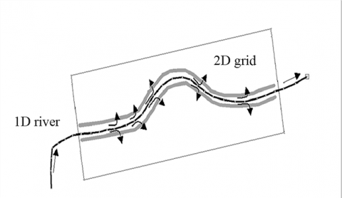
It is difficult to simulate the two-dimensional flow of uncertain path by one dimensional model, and needs long time for calculations by two dimensional model, coupled simulation of lateral connections can better take advantage of the one-dimensional model and two-dimensional models, while it can be avoid the presence of the grid resolution and accuracy of a single model problem, and to obtain even better results. Lateral connections coupled model allows two-dimensional grid connection from the side to the one-dimensional part of the river, even the entire river, Figure 1. It can be use formulas to calculate the amount of logistics structures connected by lateral flow, with lateral connections to simulate the movement of water from the river to overflow floodplain is very effective. The key is to ensure that a coupled model, at the connection point of hydraulic elements of the two-dimensional calculation area of equal value.
Figure 1. Application of lateral connection
The one-dimensional river and two-dimensional grid connected through the unified connection elevation to achieve overlapping computing unit. Connection elevation of the one-dimensional is determine by river embankment elevation, that using embankment elevation of left and right as the riverbed elevation by coupling connection, the data obtained by interpolation if it has none. Connection elevation of two-dimensional is determined by the terrain that is a two-dimensional grid cell elevation as the riverbed elevation coupling connection. Overlapping unit is setting by the hydraulic calculation nodes lap. One-dimensional computing nodes are calculation points of water level on the right and left bank river bank wire. Two dimensional compute nodes are in the grid cell corresponding to the section endpoint of right and left. Coupling model is calculate for each node dynamically conduct water, and based on water balance of node, each of the flow has been calculated re-allocated to the two-dimensional and one-dimensional computing grid cell level point, in order to achieve a one-dimensional and two-dimensional coupling calculation. One-dimensional, two-dimensional models are used in a uniform time step, and at each time step, the time will mutual exchange of information, when the water flows from one-dimensional river to two-dimensional grid, physical of computing nodes is solved by one-dimensional model as a two-dimensional model of the boundary conditions. Conversely places in the two-dimensional model of the flow value at the node, as the boundary conditions at the one-dimensional model of the connection. In order to make a stable coupling model calculation, need to ensure that the connection point of hydraulic conditions to maintain homeostasis, which requires a one-dimensional model and two-dimensional model of the initial level and flow conditions, should be the same. The two-dimensional river all the unknown variables end of the first section of the river water level linear expression, then make the flow at the end of the first boundary to boundary water form. It should be noted: coupled model just a platform model by lap one-dimensional and two-dimensional model of interactive computing, the results is still view the display on a one-dimensional river and dimensional flooded area.
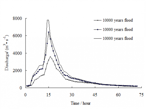
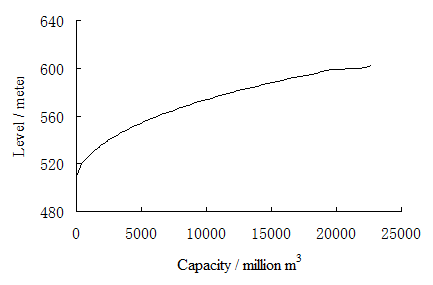
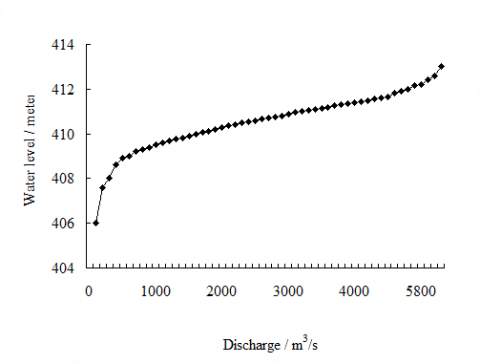
Hei river Jinpen reservoir flood control standard is design flood for 100 years (P = 1%), check flood for 2000 years (P = 0.05%), dam-break flood developed for 10,000 years (P = 0.01%) floods overtopping crashed. The inflow flood hydrograph [25] was drawn in Figure 2. The water storage capacity curve of Hei river Jinpen reservoir was shown in Figure 3. Reservoir regulation prepared for (1)when the reservoir level less than flood control level 591 m, the discharged volume is zero ; (2)when the reservoir water level between flood control level of 591 m to high water level of 594 m , the downstream flow was controlled as the incoming water flow if it is less than the allowed downstream flow of 1800 m3/s, otherwise control the discharged volume equal to 1800 m3/s; (3) when reservoir water level is greater than the high level of flood control 594 m, the gate fully open. By the flood regulating calculation on three conditions,the 100 years flood and 2000 years flood were released as flood of P=0.7% and P=0.3% years flood enter the Hei river caused dike. The 10000 years flood caused dam break when the static water level is equal to 600m at the time t = 16.4h, after spilled into the river as flood of P<0.01% (Table 1). Calculated with a gradual sloping bottom without resistance break model, the maximum dam break flow reaches 68266.95 m3/s at the time t = 17.41h, the total dam lasted 3.04h. Accordingly, drawn flow discharged line of the different frequency flood after flood routing process, shown in Figure 4.
Table 1. Condition description
|
Condition |
Inflow flood |
Outflow flood |
Burst condition |
|
Condition 1 |
P=1% |
P=0.7% |
Dike |
|
Condition 2 |
P=0.05% |
P=0.3% |
Dike |
|
Condition 3 |
P<0.01% |
P<0.01% |
Dike and dam break |
Figur 2. Reservoir inflow hydrograph
Figure 3. Relationship between water level and storage capacity
Figure 4. Reservoir outflow hydrograph
4.1 One-dimensional Simulation Conditions
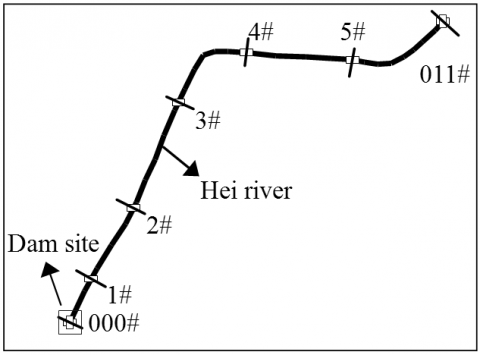
The one-dimensional simulation area of Hei river long 30920m. Selecting six sections according to the available information, the selected section were apart from dam sections 2700m, 7300m, 13700m, 19100m, 25000m, 30920m, the position is shown in Figure 5. Using the three flow processes shown in the Figure 4 as inflow boundary conditions of one-dimensional calculation. The flow water relations of section 011 # was set in Hei-Wei sink as a flow condition (Finger 6).
Figure 5. Section location
Figure 6. The discharge and water process of the Hei-Wei sink
4.2 Tne-dimensional Simulation Conditions
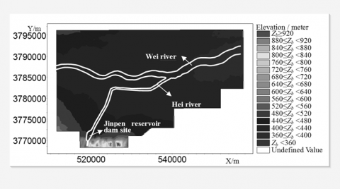
Two-dimensional calculation area includes Hei river and part of the Wei river, a total of 1 066 km2. The terrain was shown as Figure 7. Unstructured triangular grids of the different sizes were used to generation the mesh of computing area for improving accuracy. Mesh encryption processing at the river and riverbank, by controlling the density of nodes to optimize mutation border. The maximum land and river grid area were not exceeding 0.1 km2 and 0.05 km2, a total of 19 523 grids and 9974 nodes. Roughness value selecting appropriate or not have a greater impact on the calculation results, but difficult to accurately estimate due to the complexity terrain of Hei river. Roughness is generally in the range of 0.025 to 0.045, with reference to previous literature [25], and ultimately to develop a two-dimensional calculation of selected riverbed roughness value 0.031. Using the three flow processes shown in the Figure 4 as inflow boundary conditions of two-dimensional calculation. Supposing that the flow rate of y direction is zero with open outflow boundary conditions.
Figure 7. The calculation area topography of Hei river Jinpen reservoir
4.3 Coupling Model Setting
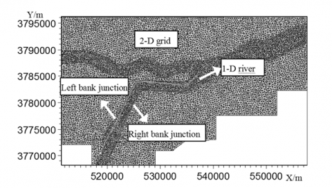
The lateral connection was used for coupled model, one-dimensional calculation section includes the entire Hei river, two-dimensional calculation part was the entire grid area, as shown in Figure 8. Both were overlapped by hydraulic calculation nodes, dam break water flows form one-dimensional river to two-dimensional region by the form of lateral weir.
Figure 8. Schematic diagram of one-dimensional and two-dimensional coupling
4.4 The Results of the Coupling Simulation
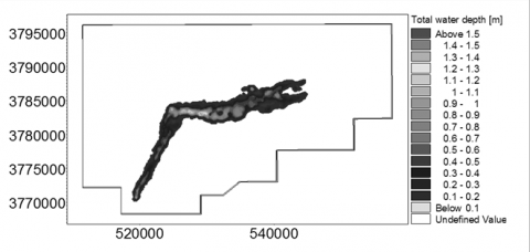
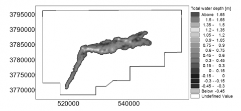
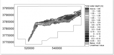
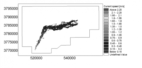
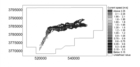
By the coupling simulation can get the instantaneous water depth and flow field distribution of the downstream flood routing, the three frequency flood submerged condition at time t=12h as an example (figure 9). Simulation lasted a total of 72h, the maximum average depth of 100,2000 and 10000 years flood occurred respectively 5.02m, 6.11m and 8.47m, the maximum average velocity were 1.97m/s, 2.14 m/s and 2.31 m/s. Coupled simulation can clear flow movement environment inside channel, and through the connecting point of interactive computing, improve the accuracy of model calculation.
(a) The water depth distribution of 100 years flood
(b) The water depth distribution of 2000 years flood
(c) The water depth distribution of 10000years flood
(d) The water velocity distribution of 100 years flood
(e) The water velocity distribution of 2000 years flood
(f) The water velocity distribution of 10000years flood
Figure 9. Instantaneous water depth and velocity distribution (t=12h)
According to the simulation results, the submergence risk map and flood velocity risk map at different frequencies and dam break flood arrival time risk map were preparation, and dam-break flood severity and risk population for analysis.
5.1 Flood Risk Map
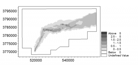
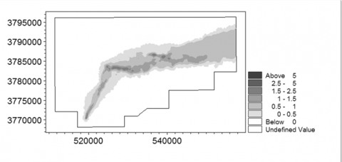
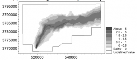
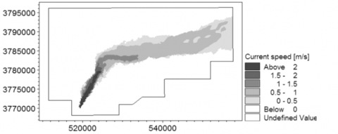
The submergence risk map and flood velocity risk map at different frequencies were shown as the figure 10. Among them, the submerged depth grading is 0~0.5 m, 0.5~1.0 m, 1.0~1.5 m, 1.5~2.5 m, 2.5~5.0 m, >5.0 m, and flood flow rate classification standard for 0~0.5 m/s, 0.5~1.0 m/s, 1.0~1.5 m/s, 1.5~2.0 m/s > 2.0 m/s.
(a) The submergence risk map of 100 years flood
(b) The submergence risk map of 2000 years flood
(c) The submergence risk map of 10000 years flood
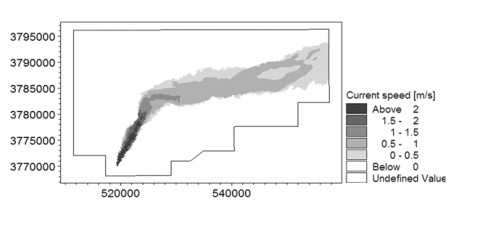
(d) The flood velocity risk map of 100 years flood
(e) The flood velocity risk map of 2000 years flood
(f) The flood velocity risk map of 10000 years flood
Figure 10. Flood risk map of different frequency floods
5.2 Dam Break Flood Risk Analysis
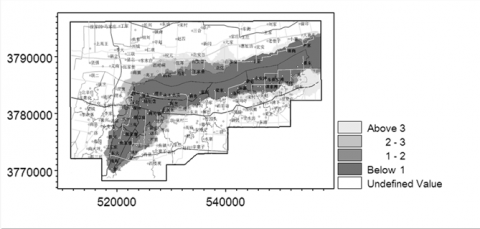
Large dam break flood water, strong currents, formed the people downstream a serious threat to the safety of life and property, seize the arrival time of the dam break flood to risk warning and evacuation of great significance. Dam break flood arrival time risk map of the 10000 years flood condition was shown as the figure 11, time grading standards for 0-1h, 1-2h, 2-3h and 3h above after dam break. Obviously, Hei river and Wei river region near have been affected in 1hour in. The affected area focused almost drowned in 3 hours. Recommend evacuation before the dam break occurred.
Figure 11. Dam break flood arrival time risk map
SD is a dam-break flood severity index, indicating the extent of the flood damage to the residents, etc., can be expressed as
$S_{D}=D \cdot V$ (5)
Where, D is the water depth, m; V is velocity, m / s.
For a grid in the i-th computing step, there is
$S_{D}=D_{\max } \cdot V_{\max } \geq \max \left(D_{i} \cdot V_{i}\right)(i=1,2, \cdots \cdots n)$ (6)
Where, Dmax for a maximum depth of the grid in the i-th step, m; Vmax is the maximum velocity of a grid in the i-th step, m/s. The safety factor of the SD value for evaluating the severity of the dam break flood is higher.
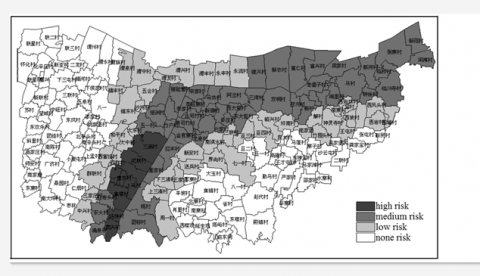
Graham method [26] divided dam break flood severity of SD types: 1) low risk, there is no flood washed away the building foundation, DV≤4.6 m2/s; 2) medium risk, flood destroyed houses generally , but the trees or destroyed houses can still provide shelter for people, 4.6 m2/s <DV≤12 m2/s; 3) high risk, flood washed away everything in the area, DV> 12 m2/s. Based on the above classification criteria, combined with the simulation results of the statistical coupling analysis, dam break flood severity distribution was shown in Figure 12. Total area affected 378.39km2, 112 villages and 257, 317 people affected, in Table 2.
Figure 12. Dam break flood severity distribution
Table 2. Dam break flood severity analysis
|
SD value (m2/s) |
severity |
Affected village |
Affected area (km2) |
Affected population(people) |
|
SD≤4.6 |
low risk |
47 |
169.34 |
130164 |
|
4.6 < SD≤12 |
medium risk |
54 |
175.85 |
109726 |
|
SD> 12 |
high risk |
11 |
33.2 |
17427 |
In this paper, the unstructured grids of non-uniform density have been used to solving model adaptive problems of complex underlying surface of mountain rivers. One-dimensional and two-dimensional hydrodynamic models have been coupled to balance calculation accuracy and efficiency by the lateral connection. The downstream flooding evolutions of different frequencies have been simulated after diking even dam breaking. The instantaneous distribution of water depth and flow field under different conditions can be shown. The maximum average depth of 100, 2000 and 10000 years flood occurred respectively 5.02m, 6.11m and 8.47m, the maximum average velocity were 1.97m/s, 2.14 m/s and 2.31 m/s. Based on the statistical analysis of the simulation results, the submergence risk map and the flood velocity risk map at different frequencies and the dam break flood arrival time risk map have been prepared and the dam-break flood severity and risk population have been analyzed. Total areas of 378.39km2, 112 villages and 257, 317 people have been affected.
This paper is supported by National Program on Key Basic Research Project (973 Program) (2012CB723201) and Central finance special funds to support local college development characteristic key subject project (Number: 106-00X101, 106-5X1205).
1. R. Choudhury and U. J. Das, Viscoelastic Effects on the Three-Dimesional Hydrodynamic Flow Past a Vertical Porous Plate, 1. International Information and Engineering Technology Association, vol. 31, pp. 1-8, 2013.
2. A. Triki and E. Hadj-Taïeb, Numerical Simulation for One Dimensional Open Channel Transient Flow, 1. International Information and Engineering Technology Association, vol. 26, pp. 87-94, 2008.
3. J. Singh and M. S. Altinakar, Two-dimensional Numerical Modeling of Dam-break Flows over Natural Terrain Using a Central Explicit Scheme, 10. Advances in Water Resources, Vol. 34, pp. 1366-13754, 2011.
4. P. Costabile and F. Macchione, Enhancing River Model Set-up for 2-D Dynamic Flood Modelling, Environmental Modelling & Software, Vol. 67, pp. 89- 107, 2015.
5. H. A. Gallegos and J. E. Schubert, Two-dimensional, High-resolution Modeling of Urban Dam- break Flooding: A Case Study of Baldwin Hills, California, 8. Advances in Water Resources, Vol. 32, pp. 1323-1335, 2009.
6. X. M. Yuan and C. F. Tian, Comprehensive Two- Dimensional Associate Hydrodynamic Models for Overflow and Levee- breach Flood and its Application,
1. Advances in Water Science, Vol. 26, pp. 83-90, 2015.
7. A. Shakibaeinia and Y. C. JIN, A Mesh-free Particle Model for Simulation of Mobile-bed Dam Break, 34. Advances in Water Resources, Vol. 6, pp. 794-807, 2011.
8. J. S. Wu and H. Zhang, Numerical Modeling of Dam- break Flood Through Intricate City Layouts Including Underground Spaces Using GPU-based SPH Method, 6. Journal of Hydraulic Engineering, Vol. 25, pp. 818- 828, 2013.
9. M. Prakash and K. Rothauge, Modelling the Impact of Dam Failure Scenarios on Flood Inundation Using SPH Original Research Article, 23. Applied Mathematical Modelling, Vol. 38, pp. 5515-5534, 2014.
10. N. B. Khedher and S. B. Nasrallah, Unstructured Control Volume Finite Element Method for Coupled Heat and Mass Transfer During the Drying of Porous Medium Having Complex 2D-geometry, 2. International Information and Engineering Technology Association, Vol. 28, pp. 77-85, 2010.
11. E. Bladé and M. Gómez-Valentín, Integration of 1D and 2D Finite Volume Schemes for Computations of Water Flow in Natural Channels, Advances in Water Resources, Vol. 42, pp. 17-29, 2012.
12. F. L. Yang and X. F. Zhang, One- and Two- Dimensional Coupled Hydrodynamics Model for Dam BreakFlow, 19. Journal of Hydraulic Engineering, Vol. 19, pp. 769-775, 2007.
13. P. Carling and I. Villanueva, Unsteady 1D and 2D Hydraulic Models with Ice Dam Break for Quaternary Megaflood, Altai Mountains, Southern Siberia, 1-4. Global and Planetary Change, Volume 70, pp. 24-34, 2010.
14. X. L. Wang and A. L. Zhang, Three-dimensional Numerical Simulation of Dam-break Flood Routing in the Complex Inundation Areas, 9. Journal of Hydraulic Engineering, Vol. 43, pp. 1025-1033, 2012.
15. W. LIU and X. D. Peng, 1-D and 2-D Coupling Numerical Simulation of Water Flow of Application in Evaluation of Flood Control, 6. China Water Transport, Vol. 10, pp. 112-113, 2010.
16. D. W. Zhang and X. T. Cheng, Dam Break Flow Mathematical Model Based on Godunov Format, 2. Advances in water science, Vol. 21, pp. 167-172, 2010.
17. X. M. Jiang and D. X. Li, 1-D and 2-D Coupled Dam Break Mathematical Model Based on the Riemann Approximate Solution, 3. Advances in Water Science, Vol. 23, pp. 214-220, 2012.
18. D. W. Zhang and J. Quan, Development and Application of 1-D Dam-break Flood Analysis System Based on GIS, 12. Journal of Hydraulic Engineering, Vol. 44, pp. 1475-1481, 2013.
19. H. h. Qi and M.S. Altinakar, A GIS-based Decision Support System for Integrated Flood Management under Uncertainty with Two Dimensional Numerical Simulations, 6. Environmental Modelling & Software, Vol. 26, pp. 817-821, 2011.
20. R. C. D. Paiva and W. Collischonn, Large Scale Hydrologic and Hydrodynamic Modeling Using Limited Data and a GIS Based Approach, 3-4. Journal of Hydrology, Vol. 406, pp. 170-181, 2011.
21. L. Jin and S. G. Xu, Flood Routing Calculation of Medium and Small Rivers Flood Risk Analysis, 10. Water Resources and Power, Vol. 32, pp. 48- 51+ 176, 2014.
22. S. M.Y. Ng and O. W. H. Wai, Integration of a GIS and a Complex Three-dimensional Hydrodynamic, Sediment and Heavy Metal Transport Numerical Model,
6. Advances in Engineering Software, Vol. 40, pp. 391- 401, 2009.
23. H. J. Liu, Research on Flood Risk Analysis Based on One-dimensional and Two-dimensional Hydraulic Coupling Calculation Model [D]. TinJin University, 2012.
24. X. H. Gu and Q. Zhang, Non-stationary Flood Risk Analysis in Pearl River Basin, Considering the Impact of Hydrological Trends, 9. Geographical Research, Vol. 33, pp. 1680-169, 2014.
25. X. D. Zhou and M. Q. Feng, Report of Hei river Jinpen Reservoir flood submerged area and evacuation plan research. Rept. Xi'an University of technology, Xi'an. 2006.
26. J. GrahamwAprocedure for estimating loss oflife caused by dam failure. Rept. Denver:U.S.Departmentof the Interior Bureau of Reclamation,1999.