Li Liu | Xindong Shi | Shuo Zhang | Yinggang Shi* | Yan Long
© 2020 IIETA. This article is published by IIETA and is licensed under the CC BY 4.0 license (http://creativecommons.org/licenses/by/4.0/).
OPEN ACCESS
Based on the hyperspectral imaging (HSI) technique, this paper attempts to test the saccharinity of three varieties of cherry tomatoes in a nondestructive manner. The cherry tomato samples of the three varieties were collected, and kept at room temperature for 12h. Then, the spectral curves of the samples were obtained between the wavelengths of 914.91nm and 1,661.91nm. After that, the feature bands were extracted by three algorithms, namely, competitive adaptive reweighted sampling (CARS), successive projection algorithm (SPA) and SPA-CARS. The samples were divided into a correction dataset and a prediction dataset at the ratio of 2:1. Next, the feature bands extracted by the three algorithms were combined with the partial least squares (PLS) and least squares-support vector machine (LS-SVM) into six saccharinity prediction models. Finally, the prediction results of the six models were compared, revealing that the CARS-LS-SVM achieved the best performance with a prediction accuracy of >92%. The evaluation indices of this model are as follows: the correlation coefficient of correction dataset ($\mathrm{R}_{c}$), 0.9696; the correlation coefficient of prediction dataset ($R_{p}$), 0.9220; the root mean square error of correction dataset (RMSEC), 0.2768; the root mean square error of prediction dataset (RMSEP), 0.4390. The research results lay the basis for industrial grading of saccharinity of cherry tomatoes in a nondestructive manner.
hyperspectral imaging (HSI), cherry tomatoes, saccharinity test, feature band extraction
Cherry tomatoes are well received by consumers, for their short maturity time, rich flavor and high nutritional value [1, 2]. The color, hardness and taste are the main considerations of cherry tomato consumers. The color and hardness of cherry tomatoes can be evaluated based on visual and hand feelings. However, it is difficult to determine the taste of the fruit, which is affected by internal qualities like saccharinity and tartness. In general, cherry tomatoes taste sour if the saccharinity is low and tartness is high, and better if the saccharinity is high and tartness is low [3]. Based on saccharinity test, it is possible to harvest and purchase cherry tomatoes in a rational manner.
Traditionally, the saccharinity of cherry tomatoes is tested destructively using a saccharimeter [4]. The destructive method is slow and inefficient. By contrast, hyperspectral imaging (HSI) features fast speed, simple operation, and good stability. The HSI is an emerging non-destructive testing (NDT) technique that combines spectral technology with imaging technology. In recent years, the HSI has developed rapidly, and been widely used to test the quality of agricultural products (APs) [5-10].
Many scholars have established APs disease detection models based on the HSI [11, 12]. For example, Abid Hussain et al. [13] created a partial least squares-discriminant analysis (PLS-DA) model based on effective attenuation coefficients, and used the model to classify tomatoes at various stages of maturity. The HIS has also been applied successfully to measure the quality, maturity and damage of fruits [14-16]. For example, Keresztes et al. [17] applied the PLS-DA model to detect the damages of apples. Combining the first derivative and mean centering, the model correctly identified 98% of damages at the pixel level, and processed each apple within 200ms. Pu et al. [18] introduced the HSI to detect the soluble solid content (SSC) of litchis. Specifically, the PSL-DA model was adopted to examine the spectral set, and the optimal wavelength was selected by the partial least squares regression (PLSR) model. Recently, the HSI has been extended to predict the SSC of apples and kiwis [19, 20]. These studies have shown the significant advantage of the HSI in the NDT of internal qualities of fruits. This technique has a promising future in food safety and APs classification [21, 22].
This paper aims to compare several HSI-based saccharinity test models for cherry tomatoes. Firstly, the HIS was adopted to obtain the spectral data of three types of cherry tomatoes. Then, the feature bands were extracted separately by three algorithms: competitive adaptive reweighted sampling (CARS), successive projection algorithm (SPA) and SPA-CARS. The three algorithms were combined with the partial least squares (PLS) and least squares-support vector machine (LS-SVM) into six saccharinity prediction models. The six models were verified by comparing their prediction results, and the optimal saccharinity prediction model was identified. The research results lay a technical basis for HSI-based saccharinity test and classification of cherry tomatoes.
2.1 Samples
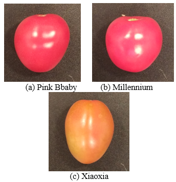
A total of 193 cherry tomato samples were collected form the greenhouses of Yangling Agricultural High-Tech Industrial Demonstration Zone, northwestern China’s Shaanxi Province. As shown in Figure 1, the samples belong to three different varieties, namely, Pink Baby, Millennium and Xiaoxia. Overall, there are 91 Pink Baby samples, 52 Millennium samples and 50 Xiaoxia samples. For convenience, every cherry tomato was given a number. To eliminate the temperature impact on prediction accuracy, the samples were kept at room temperature for 12h before obtaining their hyperspectral images [23].
Figure 1. The appearance of cherry tomato samples
2.2 Hyperspectral image acquisition system
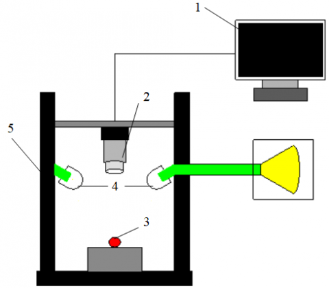
Figure 2. Hyperspectral image acquisition system
The hyperspectral images of cherry tomato samples were collected by a hyperspectral image acquisition system. As shown in Figure 2, the hyperspectral image acquisition system mainly consists of an ImSpectorN17E push-broom imaging spectrometer (Specim, Spectral Imaging Ltd., Finland) (spectral range: 900-1,700nm; sampling interval: 3.125nm; spectral resolution: 2.8nm), an XEVA3616 charge coupled device (CCD) detector, four tungsten halogen lamps (diffuse light sources; power: 100W), a working stage, a whiteboard and an image acquisition card. The entire hyperspectral image acquisition system is controlled by a computer. The SpectraSense software package was adopted to acquire the hyperspectral images.
2.3 Extraction of spectral curves
Before collecting hyperspectral images, the surface of each cherry tomato sample was cleaned. To ensure the stability of light source(s), the instruments were preheated for 30min before the samples were placed on the working stage one by one. In our experiment, nine samples are imaged at once, because the samples are relatively small and the sample location does not affect image collection. In other words, the first hyperspectral image is about samples 1-9, the second hyperspectral image is about samples 10-19, and so on in a similar fashion. The parameters of the SpectraSense software package were configured as follows: the exposure time is 11ms, the lens is vertically downward, the object distance is 200mm, and the speed of the electronically controlled stage is 12mm/s.
In addition, the collected hyperspectral images were subjected to black and white correction, aiming to reduce the noises from residual charge and uneven distribution of light intensity [24]. The correction formula can be expressed as:
$R=\frac{R_{r}-R_{d}}{R_{w}-R_{d}}$ (1)
where, $R$ is the corrected image; $R_{w}$ is the calibrated image with a reflectance close to $99.9 \%$ after scanning the standard whiteboard; $R_{d}$ is the calibrated image after turning off the light source(s); $R_{r}$ is the original hyperspectral image.
2.4 Saccharinity measurement
After collecting hyperspectral images, the saccharinity of each sample was tested by a PAL-1handheld sugar content meter. Each sample was cut horizontally; 1-3mL of juice was taken by a dropper, and dropped into the sampling tank of the meter. The true saccharinity of the sample was then read from the meter. After each test, the sampling tank was washed, and the meter was zeroed with clean water. Next, the sampling tank was cleaned with a piece of dry tissue, getting ready for the next measurement.
Table 1 lists the saccharinity of all cherry tomato samples. Obviously, there is a large difference between maximum and minimum values, and a high standard deviation, revealing the wide distribution of the sample data.
Table 1. Saccharinity of cherry tomato samples
|
Number of samples |
Saccharinity/% |
|||
|
Mean |
Minimum |
Maximum |
Standard deviation |
|
|
193 |
7.29 |
3.80 |
10.47 |
1.24 |
2.5 Division of sample set
To establish and analyze a sound saccharinity prediction model, the sample set should be divided into a correction dataset for model construction and a prediction dataset for model verification. The representativeness of the correction dataset directly bears on the performance of the prediction model. Therefore, it is necessary to select a suitable way to divide the sample set.
Being a popular tool for sample set division, the sample set partitioning based on joint x-y distances (SPXY) algorithm outperforms common approaches like random sampling (RS) and Kennard-Stone (KS) algorithm [25].
Based on the KS algorithm, the SPXY algorithm adds the two vector pairs with the longest Euclidean distance into the correction dataset, such that the samples in the correction dataset are evenly distributed in space. In the SPXY algorithm, the distances between samples p and q in the direction of spaces x and y, denoted as dx and dy, are respectively calculated by:
$d_{x}(p, q)=\sqrt{\sum_{i=1}^{I}\left[x_{p}(i)-x_{q}(j)\right]^{2}} ; p, q \in[1, N]$ (2)
$d_{y}(p, q)=\sqrt{\left(y_{p}-y_{q}\right)^{2}}=\left|y_{p}-y_{q}\right| ; p, q \in[1, N]$ (3)
Because the samples should have the same weight in the x- and y- spaces, x- and y-distances can be normalized by:
$d_{x y}(p, q)=\frac{d_{x}(p, q)}{\max _{p, q \in[1, N]} d x(p, q)}+\frac{d_{y}(p, q)}{\max _{p, q \in[1, N]} d_{y}(p, q)} ; p, q \in[1, N]$ (4)
where, $d_{x y}$ is the normalized distance between two samples.
2.6 Extraction of feature bands
There is a large amount of spectral data in the full band, many of which are redundant. The feature bands must be extracted to reduce the computing load, speed up modelling, and eliminate the impact from irrelevant variables. Therefore, this paper extracts the main bands that reflect the saccharinity features, and discards the bands that are completely or partly irrelevant to saccharinity. The extraction of feature bands reduces the dimension of variables, making the saccharinity prediction faster, more accurate and more stable.
Traditionally, feature bands are extracted by correlation coefficient method, principal component analysis (PCA), genetic algorithm (GA, and stepwise regression analysis method. After years of perfection, these methods have become very mature. Recently, two emerging algorithms, namely, CARS and SPA, have been successfully applied to extract feature bands.
The CARS algorithm can effectively select a subset of variables containing abundant information, which is conductive to model simplification. The subset is selected in two steps: computing the root-mean-square error of cross-validation (RMSECV) of each subset; comparing the RMSECVs of all subsets; taking the subset with the smallest RMSECV as the target subset.
The SPA, as a forward loop-based variable filtering algorithm, can reduce the collinearity of vector space between variables, and effectively prevent information overlap and redundancy. The extracted feature bands have a low collinearity, represent rich information with little information, and thus ease the computing load.
However, both CARS and SPA extract a large number of feature wavelengths. To simplify the model and improve computing efficiency, this paper decides to select feature bands in two steps: extracting 40 feature bands by the SPA, followed by CARS extraction from the 40 bands. The optimal plan for feature band extraction was then determined through RMSECV comparison.
2.7 Modelling method and evaluation indices
This paper sets up the PLS model and LS-SVM model for saccharinity prediction based on three different methods for feature band extraction: CARS, SPA and SPA-CARS [26].
The PLS fully combines the merits of principal component analysis (PCA), multiple linear regression (MLR) and canonical correlation analysis (CCA). It can solve many problems that cannot be handled by common regression models. By the PLS, the best mapping relationship between the dependent variable and the independent variable is found based on the least sum of squares for error (SSE). Then, a small part of the variables that represents the collinearity of most information is identified for regression analysis and modeling. In the PLS, the number of principal components means the number of combinations of weighted feature spectral data.
Based on the SVM and PLS, the LS-SVM is a kernel-based learning technique capable of solving both linear and nonlinear regression problems. The main principle is to transform the input variables into a high-dimensional feature space through nonlinear mapping, and establish the best regression function in the space. The key of the LS-SVM modelling lies in the selection of kernel functions and kernel parameters. Different choices directly affect the performance of the LS-SVM model. In this paper, radial basis function (RBF) is taken as the kernel function of the LS-SVM to reduce the computing complexity in the modelling process.
In the course of modelling, the sample set was first divided into a correction dataset and a prediction dataset. The former is used for modelling and the latter for model evaluation. The results of the two datasets demonstrate the modelling effect. In this paper, the models are evaluated by the following indices: correlation coefficient of correction dataset $\left(\mathrm{R}_{c}\right),$ root mean square error of correction dataset (RMSEC), correlation coefficient of prediction dataset ($\mathrm{R}_{p}$), and root mean square error of prediction dataset (RMSEP). In general, the greater the $\mathrm{R}$ value, the smaller the RMSE, and the better the prediction effect. The maximum value of $\mathrm{R}$ is $1,$ and the minimum value of RMSE is 0.
3.1 Spectral features of samples
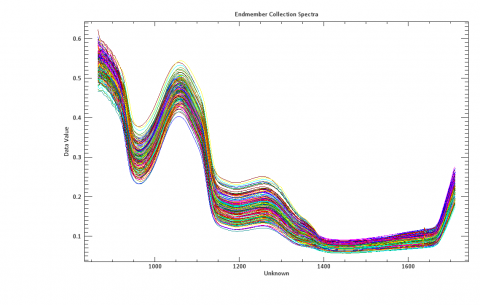
The full spectrum curves of 193 cherry tomato samples are displayed in Figure 3, where the abscissa is the wavelength and the ordinate are the spectral value. For each sample, 256 spectral values were extracted from the 256 bands, and represented as a spectral curve in Figure 3. The smoothness of the curves demonstrates that the spectral data contain a low level of noises, and are not greatly disturbed. The spectral curves of these samples were similar in shape, indicating that there are no abnormal samples. Moreover, the spectrum curves were not smooth in the front, a sign of the presence of noises, and bended up at the tail. Hence, the spectrum data of the first and last 15 bands were removed, leaving those of the 226 bands between 914.91nm and 1,661.9nm for further processing.
Figure 3. Spectral curves of samples
3.2 Division of sample set
For the universality of modeling, the SPXY algorithm was adopted to divide the samples of each variety into a correction dataset and a prediction dataset at the ratio of 2:1. The correction dataset contains 130 samples, including 61 of Pink Baby, 35 of Millennium and 34 of Xiaoxia.
Table 2. The saccharinity data in the correction dataset and the prediction dataset
|
Dataset |
Number of samples |
Saccharinity % |
|||
|
Mean |
Minimum |
Maximum |
Standard deviation |
||
|
Correction dataset |
130 |
7.26 |
3.80 |
10.47 |
1.31 |
|
Prediction dataset |
63 |
7.35 |
4.97 |
9.80 |
1.1 |
Table 2 presents the saccharinity data in the correction dataset and the prediction dataset. The large standard deviation of the correction dataset reflects that the data cover a wide range, which is good for modelling.
3.3 Results of feature band extraction
3.3.1 CARS
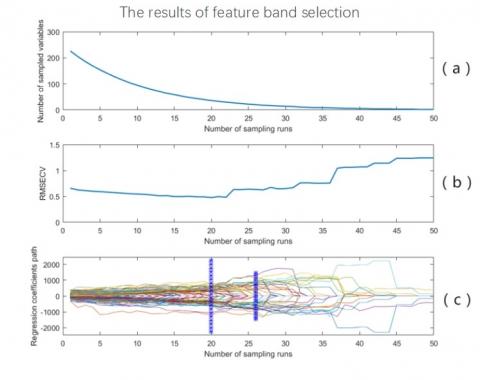
The feature bands were extracted after data normalization. The number of sampling runs was set to 50. The feature bands selected by CARS are shown in Figure 4, where (a) (b) and (c) are the variations in the number of variables, the RMSECV, and the regression coefficient with the sampling runs, respectively. The minimum RMSECV (0.4789%) appeared in the 20th sampling run, between the star lines in (c). In this case, 36 wavelength variables were retained. Table 3 lists the 36 wavelengths extracted from the 226 bands.
Figure 4. Feature bands extracted by CARS
Table 3. The 36 wavelengths extracted by CARS
|
Serial number |
Wavelength |
Serial number |
Wavelength |
Serial number |
Wavelength |
Serial number |
Wavelength |
Serial number |
Wavelength |
|
1 |
934.83nm |
9 |
1,001.23nm |
17 |
1,120.75nm |
25 |
1,293.39nm |
33 |
1,602.15nm |
|
2 |
941.47nm |
10 |
1,007.87nm |
18 |
1,130.71nm |
26 |
1,139.87nm |
34 |
1,625.39nm |
|
3 |
944.79nm |
11 |
1,014.51nm |
19 |
1,163.91nm |
27 |
1,363.11nm |
35 |
1,645.31nm |
|
4 |
951.43nm |
12 |
1,017.83nm |
20 |
1,177.19nm |
28 |
1,456.07nm |
36 |
1,651.95nm |
|
5 |
954.75nm |
13 |
1,044.39nm |
21 |
1,180.51nm |
29 |
1,539.07nm |
|
|
|
6 |
984.63nm |
14 |
1,047.71nm |
22 |
1,187.15nm |
30 |
1,542.39nm |
|
|
|
7 |
987.95nm |
15 |
1,084.23nm |
23 |
1,220.35nm |
31 |
1,555.67nm |
|
|
|
8 |
997.91nm |
16 |
1,100.83nm |
24 |
1,236.95nm |
32 |
1,578.91nm |
|
3.3.2 SPA
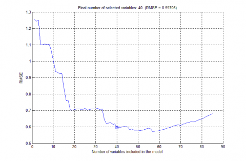
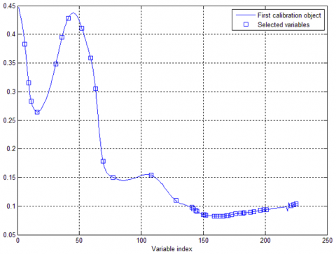
The interval of valid wavelengths must be determined before extracting feature bands by the SPA. Here, the lower bound of the valid number of wavelengths is fixed at 1, while the upper bound is changed continuously from 5 at the step length of 5. In other words, the interval of the number of valid wavelengths was changed from 1-5, 1-10, 1-15 to 1-20. As shown in Figure 5, the minimum RMSE (0.59706%) was observed under the interval of 1-50. The number of wavelengths (40) corresponding to the minimum RMSE was taken as the optimal number of wavelengths. The 40 feature wavelengths extracted from the 226 bands are listed in Table 4, and their distribution is illustrated in Figure 6.
Figure 5. The relationship between RMSE and number of feature bands extracted by the SPA
Figure 6. Feature bands extracted by SPA
Table 4. The 40 feature bands extracted by SPA
|
Serial number |
Wavelength |
Serial number |
Wavelength |
Serial number |
Wavelength |
Serial number |
Wavelength |
Serial number |
Wavelength |
|
1 |
931.51nm |
9 |
1,107.46nm |
17 |
1,389.67nm |
25 |
1,462.71nm |
33 |
1,535.75nm |
|
2 |
941.47nm |
10 |
1,120.75nm |
18 |
1,392.99nm |
26 |
1,472.67nm |
34 |
1,545.71nm |
|
3 |
948.11nm |
11 |
1,140.67nm |
19 |
1,409.59nm |
27 |
1,475.99nm |
35 |
1,562.31nm |
|
4 |
964.71nm |
12 |
1,167.23nm |
20 |
1,412.91nm |
28 |
1,485.95nm |
36 |
1,572.27nm |
|
5 |
1,014.51nm |
13 |
1,270.15nm |
21 |
1,416.23nm |
29 |
1,495.91nm |
37 |
1,578.91nm |
|
6 |
1,031.11nm |
14 |
1,336.55nm |
22 |
1,439.47nm |
30 |
1,509.19nm |
38 |
1,645.31nm |
|
7 |
1,047.71nm |
15 |
1,379.71nm |
23 |
1,446.11nm |
31 |
1,515.83nm |
39 |
1,651.95nm |
|
8 |
1,084.23nm |
16 |
1,383.03nm |
24 |
1,456.07nm |
32 |
1,519.15nm |
40 |
1,658.59nm |
3.3.3 SPA-CARS
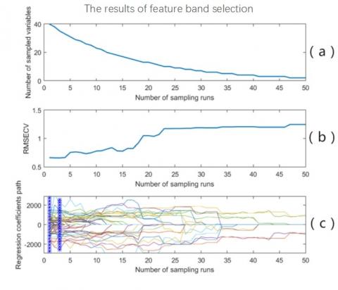
As mentioned before, both CARS and SPA extract a large number of feature wavelengths. To simplify the model and improve computing efficiency, the feature bands were further selected in two steps: extracting 40 feature bands by the SPA, followed by CARS extraction from the 40 bands. The number of sampling runs was still set to 50. The feature bands extracted by SPA-CARS are presented in Figure 7, where (a) (b) and (c) are the variations in the number of variables, the RMSECV, and the regression coefficient with the sampling runs, respectively. The minimum RMSECV (0.6611%) appeared in the 3rd sampling run. A total of 35 feature bands (Table 5) was retained between the star lines.
Figure 7. Feature bands extracted by SPA-CARS
Table 5. The 35 feature bands extracted by SPA-CARS
|
Serial number |
Wavelength |
Serial number |
Wavelength |
Serial number |
Wavelength |
Serial number |
Wavelength |
Serial number |
Wavelength |
|
1 |
931.51nm |
8 |
1,084.23nm |
15 |
1,383.03nm |
22 |
1,462.71nm |
29 |
1,535.75nm |
|
2 |
941.47nm |
9 |
1,107.46nm |
16 |
1,389.67nm |
23 |
1,472.67nm |
30 |
1,545.71nm |
|
3 |
948.11nm |
10 |
1,120.75nm |
17 |
1,409.59nm |
24 |
1,475.99nm |
31 |
1,572.27nm |
|
4 |
964.71nm |
11 |
1,140.67nm |
18 |
1,412.91nm |
25 |
1,485.95nm |
32 |
1,578.91nm |
|
5 |
1,014.51nm |
12 |
1,167.23nm |
19 |
1,416.23nm |
26 |
1,495.91nm |
33 |
1,645.31nm |
|
6 |
1,031.11nm |
13 |
1,270.15nm |
20 |
1,446.11nm |
27 |
1,515.83nm |
34 |
1,651.95nm |
|
7 |
1,047.71nm |
14 |
1,336.55nm |
21 |
1,456.07nm |
28 |
1,519.15nm |
35 |
1,658.59nm |
Compared with one-step extraction methods (SPA and CARS), the two-step extraction method (SPA-CARS) extracted a relatively few feature bands and had a relatively high RMSE. This means the high computing efficiency (and limited number of feature bands) of SPA-CARS comes at the cost of model accuracy. Further analysis is needed to compare the modelling effects of the feature bands extracted by the three methods.
3.4 Model results
3.4.1 Results of PLS models
The PLS algorithm was introduced to create a saccharinity prediction model based on the feature bands obtained by each of the three extraction methods. Table 6 compares the performance of the three resulting models. For simplicity, the PLS models based on the feature bands extracted by CARS, SPA and SPA-CARS are denoted as CARS-PLS, SPA-PLS, and SPA-CARS-PLS, respectively.
It can be seen that the CARS-PLS performed well in correction and prediction, for it achieved the largest $R_{c}$ and smallest RMSEC in both correction dataset and prediction dataset. Meanwhile, the SPA-CARS-PLS performed less well in correction and prediction, but consumed a shorter time, than the CARS-PLS. Hence, SPA-CARS-PLS sacrifices the model performance for computing speed.
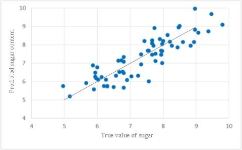
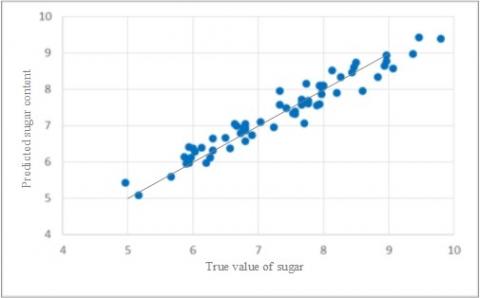
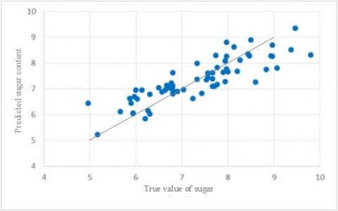
The scatter plots of saccharinity predicted by the three models are displayed in Figure 8, where the abscissa is the true saccharinity of the 63 prediction samples, and the ordinate is the predicted saccharinity. The linearity of the distribution of scatter points is positively correlated with the prediction accuracy of the corresponding model. It is clear that the CARS-PLS had the best prediction performance. By the simplex method, the suitable parameters were selected as $\gamma=72,385$ and $\sigma^{2}=252$.
Table 6. Performance comparison between PLS models
|
Extraction method |
Number of feature bands |
$\mathbf{R}_{\mathbf{c}}$ |
RMSEC/Saccharinity |
$\mathbf{R}_{\mathbf{p}}$ |
RMSEP/Saccharinity |
|
CARS |
36 |
0.9163 |
0.5253 |
0.8706 |
0.5753 |
|
SPA |
40 |
0.9030 |
0.5638 |
0.8385 |
0.6487 |
|
SPA-CARS |
35 |
0.8870 |
0.6076 |
0.8195 |
0.6982 |
3.4.2 Results of LS-SVM models
Next, the LS-SVM algorithm was introduced to create a saccharinity prediction model based on the feature bands obtained by each of the three extraction methods. Table 7 compares the performance of the three resulting models. For simplicity, the LS-SVM models based on the feature bands extracted by CARS, SPA and SPA-CARS are denoted as CARS-LS-SVM, SPA-LS-SVM, and SPA-CARS-LS-SVM, respectively.
Table 7. Performance comparison between LS-SVM models
|
Extraction method |
Number of feature bands |
$\mathbf{R}_{\mathbf{c}}$ |
RMSEC/Saccharinity |
$\mathbf{R}_{\mathbf{p}}$ |
RMSEP/Saccharinity |
|
CARS |
36 |
0.9696 |
0.2768 |
0.9220 |
0.4390 |
|
SPA |
40 |
0.9504 |
0.4140 |
0.8871 |
0.5188 |
|
SPA-CARS |
35 |
0.9434 |
0.4390 |
0.8850 |
0.5231 |
It can be seen that the CARS-PLS still performed well in correction and prediction, with the largest $\mathrm{R}_{\mathrm{c}}$ and smallest RMSEC. The three LS-SVM models differed slightly in results. Their $R_{c}$ values were all greater than $0.94,$ and their $R_{p}$ values were all above 0.88. These results demonstrate the excellent modelling effect of LS-SVM. However, the LS-SVM modelling takes a relatively long time, averaging at around 200s.
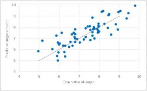
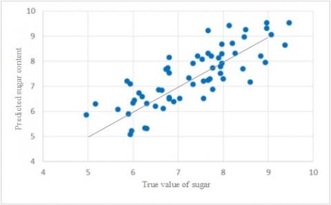
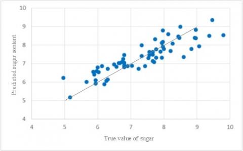
The scatter plots of saccharinity predicted by the three models are displayed in Figure 9, where the abscissa is the true saccharinity of the 63 prediction samples, and the ordinate is the predicted saccharinity. Comparing the three subgraphs, it can be seen that the distribution of saccharinity predicted by the CARS-LS-SVM was more similar to a straight line than that predicted by the other two models. Hence, the CARS-LS-SVM boasts the best prediction effect among the three LS-SVM models.
(a) CARS-PLS
(b) SPA-PLS
(c) SPA-CARS-PLS
Figure 8. Scatter plots of saccharinity predicted by PLS models
(a) CARS-LS-SVM
(b) SPA-LS-SVM
(c) SPA-CARS-LS-SVM
Figure 9. Scatter plots of saccharinity predicted by LS-SVM models
The three PLS models and the three LS-SVM models were further compared in terms of correction performance and prediction performance. As shown in Table 8, the CARS-LS-SVM achieved the best (0.9220), (0.9696), RMSEC (0.2768) and RMSEP (0.4390) among all the six models. Besides, the PLS models all surpassed the LS-SVM models in correlation coefficient, i.e. the LS-SVM models are better in accuracy.
Table 8. Performance comparison between the six models
|
Extraction method |
Modelling method |
Number of feature bands |
$\mathbf{R}_{c}$ |
RMSEC/Saccharinity |
$\mathbf{R}_{p}$ |
RMSEP/Saccharinity |
|
CARS |
PLS |
36 |
0.9163 |
0.5253 |
0.8706 |
0.5753 |
|
LS-SVM |
0.9696 |
0.2768 |
0.9220 |
0.4390 |
||
|
SPA |
PLS |
40 |
0.9030 |
0.5638 |
0.8385 |
0.6487 |
|
LS-SVM |
0.9504 |
0.4140 |
0.8871 |
0.5188 |
||
|
SPA-CARS |
PLS |
35 |
0.8870 |
0.6076 |
0.8195 |
0.6982 |
|
LS-SVM |
0.9434 |
0.4390 |
0.8850 |
0.5231 |
Based on the HSI, this paper explores the saccharinity test models of cherry tomatoes. Three extraction methods, namely, CARS, SPA and SPA-CARS, were adopted to extract the feature bands from 226 bands in the spectral curves of all cherry tomato samples. Then, the PLS and LS-SVM were separately introduced to create saccharinity prediction models based on the feature bands extracted by the above three algorithms. Comparison shows that the CARS-LS-SVM model achieved the best prediction effect, as evidenced by its (0.9220), (0.9696), RMSEC (0.2768) and RMSEP (0.4390). Under the same conditions, the LS-SVM models have greater correlation coefficient and better accuracy in prediction than the PLS models. The research results lay the basis for industrial grading of saccharinity of cherry tomatoes in a nondestructive manner.
This work is supported by the Shaanxi Key Research and Development Program of China (Grant numbers: 2019NY-171, 2019ZDLNY02-04, 2018TSCXL-NY-05-04). The authors are also gratefully to the reviewers for their helpful comments and recommendations, which make the presentation better.
[1] Buendia-Moreno, L., Soto-Jover, S., Ros-Chumillas, M., Antolinos, A., Navarro−Segura, L., Sánchez−Martínez, M.J., Martínez−Hernández, G.B., López−Gómez, A. (2019). Innovative cardboard active packaging with a coating including encapsulated essential oils to extend cherry tomato shelf life. LWT-Food Science and Technology, 116: 108584. https://doi.org/10.1016/j.lwt.2019.108584
[2] Liu, H., Meng, F., Miao, H., Chen, S., Yin, T., Hu, S., Shao, Z., Liu, Y., Gao, L., Zhu, C., Zhang, B., Wang, Q. (2018). Effects of postharvest methyl jasmonate treatment on main healthpromoting components and volatile organic compounds in cherry tomato fruits. Food Chemistry, 263, 194-200. https://doi.org/10.1016/j.foodchem.2018.04.124
[3] Schouten, R.E., Woltering, E.J., Tijskens, L.M.M. (2016). Sugar and acid interconversion in tomato fruits based on biopsy sampling of locule gel and pericarp tissue. Postharvest Biology and Technology, 111: 83-92. https://doi.org/10.1016/j.postharvbio.2015.07.032
[4] Truffault, V., Gest, N., Garchery, C., Florian, A., Fernie, A.R., Gautier, H., Stevens, R.G. (2016). Reduction of MDHAR activity in cherry tomato suppresses growth and yield and MDHAR activity is correlated with sugar levels under high light. Plant, Cell & Environment, 39(6): 1279-1292. https://doi.org/10.1111/pce.12663
[5] Pathmanaban, P., Gnanavel, B.K., Anandan, S.S. (2019). Recent application of imaging techniques for fruit quality assessment. Trends in Food Science & Technology, 94: 32-42. https://doi.org/10.1016/j.tifs.2019.10.004
[6] Chandrasekaran, I., Panigrahi, S.S., Ravikanth, L., Singh, C.B. (2019). Potential of Near-Infrared (NIR) spectroscopy and hyperspectral imaging for quality and safety assessment of fruits: An overview. Food Analytical Methods, 12(11): 2438-2458. https://doi.org/10.1007/s12161-019-01609-1
[7] Ding, X.B., Zhang, C., Liu, F., Song, X.L., Kong, W.W., He, Y. (2015). Determination of soluble solid content in strawberry using hyperspectral imaging combined with feature extraction methods. International Journal of Analytical Chemistry, 35(4): 1020-1024.
[8] Peng, Y., Lu, R. (2008). Analysis of spatially resolved hyperspectral scattering images for assessing apple fruit firmness and soluble solids content. Postharvest Biology and Technology, 48(1): 52-62. https://doi.org/10.1016/j.postharvbio.2007.09.019
[9] Hu, W., Sun, D.W., Blasco, J. (2017). Rapid monitoring 1-MCP-induced modulation of sugars accumulation in ripening ‘Hayward’kiwifruit by Vis/NIR hyperspectral imaging. Postharvest Biology and Technology, 125: 168-180. https://doi.org/10.1016/j.postharvbio.2016.11.001
[10] Zhang, D., Xu, L., Liang, D., Xu, C., Jin, X., Weng, S. (2018). Fast prediction of sugar content in dangshan pear (Pyrus spp.) using hyperspectral imagery data. Food Analytical Methods, 11(8): 2336-2345. https://doi.org/10.1007/s12161-018-1212-3
[11] Lu, J., Zhou, M., Gao, Y., Jiang, H. (2018). Using hyperspectral imaging to discriminate yellow leaf curl disease in tomato leaves. Precision Agriculture, 19(3): 379-394. https://doi.org/10.1007/s11119-017-9524-7
[12] Femenias, A., Gatius, F., Ramos, A.J., Sanchis, V., Marín, S. (2019). Use of hyperspectral imaging as a tool for Fusarium and deoxynivalenol risk management in cereals: A review. Food Control, 108: 106819. https://doi.org/10.1016/j.foodcont.2019.106819
[13] Hussain, A., Pu, H., Sun, D.W. (2019). Measurements of lycopene contents in fruit: A review of recent developments in conventional and novel techniques. Critical Reviews in Food Science and Nutrition, 59(5): 758-769. https://doi.org/10.1080/10408398.2018.1518896
[14] Wang, H., Zhang, R., Peng, Z., Jiang, Y., Ma, B. (2019). Measurement of SSC in processing tomatoes (Lycopersicon esculentum Mill.) by applying Vis‐NIR hyperspectral transmittance imaging and multi‐parameter compensation models. Journal of Food Process Engineering, 42(5): e13100. https://doi.org/10.1111/jfpe.13100
[15] Rahman, A., Park, E., Bae, H., Cho, B. K. (2018). Hyperspectral imaging technique to evaluate the firmness and the sweetness index of tomatoes. Korean Journal of Agricultural Science, 45(4): 823-837.
[16] Zhang, C., Guo, C., Liu, F., Kong, W., He, Y., Lou, B. (2016). Hyperspectral imaging analysis for ripeness evaluation of strawberry with support vector machine. Journal of Food Engineering, 179: 11-18. https://doi.org/10.1016/j.jfoodeng.2016.01.002
[17] Keresztes, J.C., Goodarzi, M., Saeys, W. (2016). Real-time pixel based early apple bruise detection using short wave infrared hyperspectral imaging in combination with calibration and glare correction techniques. Food Control, 66: 215-226. https://doi.org/10.1016/j.foodcont.2016.02.007
[18] Pu, H., Liu, D., Wang, L., Sun, D.W. (2016). Soluble solids content and pH prediction and maturity discrimination of lychee fruits using visible and near infrared hyperspectral imaging. Food Analytical Methods, 9(1): 235-244. https://doi.org/10.1007/s12161-015-0186-7
[19] Fan, S., Zhang, B., Li, J., Liu, C., Huang, W., Tian, X. (2016). Prediction of soluble solids content of apple using the combination of spectra and textural features of hyperspectral reflectance imaging data. Postharvest Biology and Technology, 121: 51-61. https://doi.org/10.1016/j.postharvbio.2016.07.007
[20] Guo, W., Zhao, F., Dong, J. (2016). Nondestructive measurement of soluble solids content of kiwifruits using near-infrared hyperspectral imaging. Food Analytical Methods, 9(1): 38-47. https://doi.org/10.1007/s12161-015-0165-z
[21] Khan, M.J., Khan, H.S., Yousaf, A., Khurshid, K., Abbas, A. (2018). Modern trends in hyperspectral image analysis: A review. IEEE Access, 6, 14118-14129. https://doi.org/10.1109/ACCESS.2018.2812999
[22] Li, S., Song, W., Fang, L., Chen, Y., Ghamisi, P., Benediktsson, J.A. (2019). Deep learning for hyperspectral image classification: An overview. IEEE Transactions on Geoscience and Remote Sensing, 57(9): 6690-6709. https://doi.org/10.1109/TGRS.2019.2907932
[23] Li, R., Fu, L. (2017), Nondestructive measurement of sugar and hardness of blueberry based on hyperspectral image. Transactions of the Chinese Society of Agricultural Engineering, 33: 362-366. https://doi.org/10.11975/j.issn.1002-6819.2017.z1.054
[24] Ma, T., Li, X., Inagaki, T., Yang, H., Tsuchikawa, S. (2018). Noncontact evaluation of soluble solids content in apples by near-infrared hyperspectral imaging. Journal of Food Engineering, 224: 53-61. https://doi.org/10.1016/j.jfoodeng.2017.12.028
[25] Wang, S.F., Han, P., Cui, G.L., Wang, D., Liu, S.S., Zhao, Y. (2019). Near-infrared spectroscopy of watermelon soluble solids using SPXY algorithm. Spectroscopy and Spectral Analysis, 39(3): 738-742.
[26] Zhou, Z., Morel, J., Parsons, D., Kucheryavskiy, S.V., Gustavsson, A.M. (2019). Estimation of yield and quality of legume and grass mixtures using partial least squares and support vector machine analysis of spectral data. Computers and Electronics in Agriculture, 162: 246-253. https://doi.org/10.1016/j.compag.2019.03.038