Salim Kerai*![]() | Youcef Hamoudi
| Youcef Hamoudi
© 2023 IIETA. This article is published by IIETA and is licensed under the CC BY 4.0 license (http://creativecommons.org/licenses/by/4.0/).
OPEN ACCESS
The quantification of electrical conductivity in fluids is integral to various applications, including water engineering, biomedical, and industrial sectors. This study introduces an innovative methodology harnessing phase-sensitive detection to assess conductance, thereby nullifying the coupling capacitances' interference between the probe cell's metallic electrodes. The devised electronic conditioning circuit incorporates a 1 kHz sinusoidal voltage source, an admittance-to-voltage converter, a lock-in amplifier, and a microcontroller/LCD interface. Calibrations were performed over two ranges, 1 mS/cm and 20 mS/cm, utilizing precise combinations of resistors, capacitors, and adjustable resistors. The experimental findings were juxtaposed with a standard commercial conductometer across various solutions - calibration solutions, electrolyte solutions (NaCl, KCl, CaCl2, MgSO4), and different water treatment room solutions at a hemodialysis center (Carbon filter, water softener, Reverse osmosis, Dialysate). The relative error in the measured conductivity was derived, with a maximum value of 1.45% noted. This error margin is inferior to those reported by many commercial conductivity meters, suggesting improved accuracy of our method.
electrical conductivity, probe cell, capacitive influence, phase sensitive detection, conductance, lock-in amplifier, calibration, standard solution, precision resistor
The electrical conductivity is one of basic electrical parameters of fluids and solids. The measurement of this parameter is very important for water, industrial and biomedical engineering to provide information about ions concentration. Thus, the density of electrical conducting materials is determined indirectly from measurements of electrical conductivity.
In water treatment, it is used for monitoring demineralization process. In electrowinning, the conductivity of the electrolyte directly influences the quality of the primary metal related to current efficiency [1].
In battery industry, the design of cells and thermal balance is enhanced by measuring the electrical conductivity of the electrolyte [2].
In food industry, electrical conductivity measurement is related to food characteristics such as free water and contents concentration [3]. For example, the concentration of monosodium glutamate (MSG) is evaluated by electrical conductivity to study these effects on the body's organs [4].
In geotechnical engineering, electrical conductivity sensors have been used for monitoring correlation of changes in soil conductivity and water content during cyclic wetting and drying of the soil [5].
In biomedical engineering, biological parameters are explored via electrical conductivity such as skin and blood plasma. In hemodialysis applications, it is used for monitoring the concentration of solutions in water treatment room and the dialysate in dialysis machine [6].
The conductivity σ is extracted from conductance G of a probe cell based on metal electrodes. This conductance corresponds to an alternating (sinusoidal or square) voltage VS applied between electrodes in order to generate the electric current IS given by Ohm’s law:
$V_S=R I_S$ (1)
or
$I_S=G V_S$ (2)
where the conductance G is the reciprocal of the resistance R of probe cell.
The electric field between electrodes due to voltage VScauses the ions of solution to move back and forth with conductance G producing an alternating current IS.
Electrical conductivity is directly calculated from a measurement of the corresponding conductance G. In the case of homogeneous dimensions G is given by:
$G=\sigma \frac{A}{d}=\sigma K$ (3)
with
$K=\frac{A}{d}$ (4)
then
$\sigma=K\, G$ (5)
where σ is the electrical conductivity, d is the distance between the electrodes, A is their section, and K is the cell constant. In the case when the effective cross-section of the cell A is variable with d, a cell constant has also an invariable value K. In general, this value must not be calculated by geometric dimensions of cell due to the leakage of the electric field at the ends of the electrode plates. It must be determined by a calibration with standard liquid of known conductivity. Note that electrodes of probe cell are generally based on titanium or stainless steel which are more effective than graphite and platinum [7].
The aim of the present work is to propose a new device to eliminate the problems encountered in many conditioning techniques. This device measures electrical conductivity σ based on a 1 kHz single sinusoidal source, an admittance to voltage converter and a lock-in amplifier using a technique known as phase sensitive detection to eliminate electrodes/solution capacitance. A microcontroller is used to calculate electrical conductivity and send his value to LCD for display.
The precision resistors in parallel with capacitors were used to simulate electrical conductivity and calibrate the proposed device by using adjustable precision resistors to achieve accuracy of 1.45% which is generally 2% in commercial conductivity meters. Finally, the experimental results obtained by different solutions are showed and discussed.
The role of conditioning circuits is to extract the value of conductance G because it is directly related to Electrical conductivity σ (Eq. (5)). The most conditioning circuits used for measuring the conductance G are the bridge techniques like Wheatstone bridge which must verify equilibrium conditions.
Generally, the electrodes/solution system is represented by complex admittance that is a conductance G (real part) in parallel with capacitance C (imaginary part). Different transformer bridges are used for measuring the phase shift between the current and voltage in probe cell with the aim to eliminate capacitive current injected in complex admittance [8-11].
These bridge techniques are not able to measure rapid variations of conductivity and rapid changes in solution concentration because the measurement requires the balancing of the bridges for fixed values of passive components (resistors and capacitors) constituting of the bridge. The precision of measurement of conductivity is limited by the accuracy of the value of passive components.
By using square-wave source and Fourier transforms calculations, the conductance G can be estimated from complex admittance. This method measures rapid changes in conductivity but it requires complex programs and it is difficult to implement this solution in compact device [12].
The proposed device is capable to measure rapid changes of conductivity by using an admittance to voltage converter which does not require equilibrium conditions. A lock-in amplifier is used to eliminate capacitive influence of electrodes/solution system and extract value of conductance G from complex admittance. A simple program is implemented in microcontroller to calculate electrical conductivity.
The Figure 1 shows the block diagram of proposed electrical conductivity meter with two measurement ranges of conductivity σ (20 mS/cm and 1 mS/cm) and accuracy of 1.45%. The proposed device consists of a sinusoidal voltage source, an admittance to voltage converter, a phase detection sensitive stage and microcontroller/LCD card.
Figure 1. Block diagram of proposed device
The voltage source is an oscillator that produces a signal whose frequency f is 1 kHz at constant amplitude (VSR or VSR2). This signal is the input of the admittance to voltage converter which provides an output sinusoidal voltage $\bar{V}_Y$ proportional to complex admittance $\bar{Y}$ of solution/electrodes system that is composed of conductance G with parallel of capacitor C. Thus,
$\bar{V}_Y=\bar{K}_Y \bar{Y}$ (6)
where, $\bar{K}_Y$ is the conversion factor and $\bar{Y}$ is given by:
$\bar{Y}=G+j 2 \pi f C$ (7)
The output signal of this converter is applied to the phase sensitive detection based on lock-in amplifier to extract a conductance G from $\bar{Y}$.
The output signal is DC voltage which is proportional to value of G. This DC voltage is given by:
$V_G=K_G G$ (8)
where, KG is the factor that depends on components of lock-in amplifier consisting of an analog multiplier followed by a lowpass filter.
The voltage VG is converted to the electrical conductivity σ from K cell constant by microcontroller using equation:
$\sigma=K \,G$ (9)
This microcontroller is also used to select two measurement ranges of σ (20 mS/cm and 1 mS/cm) and display on LCD the calculated electrical conductivity.
4.1 The sinusoidal voltage source
The use of the sinusoidal voltage source allows to avoid the electrolysis of solution which generates errors in measured electrical conductivity as the case of DC polarization. On the other hand, this source is applied to probe cell and serves as the reference to lock-in amplifier. As a result, the phase shift between the output of admittance to voltage converter and the lock-in reference corresponds to the phase of admittance $\bar{Y}$.
Figure 2. Sinusoidal voltage source
The configuration of sinusoidal voltage source is shown in Figure 2. It uses a sinusoidal oscillator based on XR-2206 that is a function generator integrated circuit capable of producing stable output waveforms (sine, square, triangle, ramp) with low total harmonic distortion and amplitude and frequency adjusted by external resistors making it appropriate for the designed device.
Frequency of operation can be selected over a range of 0.01 Hz to more than 1 MHz and can be adjusted by the external capacitor, C1, across Pin 5 and 6, and by the resistor, R2, connected to either Pin 7 or 8. The frequency is given as [13]:
$f=\frac{1}{R_2 C_1}$ (10)
Output sinusoidal amplitude (pin 2 of XR2206) is directly proportional to the adjustable resistance RV1 connected on pin 3 of XR2206.
The DC level at the output (pin 2 of XR2206) is approximately the same as the DC bias at Pin 3. This DC level which is not suitable for polarization of cell probe is removed by first order passive high-pass filter RV2C3. The cutoff frequency is given as:
$f_H=\frac{1}{2 \pi R_{V 2} C_3}$ (11)
This filter has two sinusoidal outputs. The first (pin 2 of RV2) is used as the reference signal $\bar{V}_{S R}$ in lock-in amplifier and is adjusted by RV1. The second (pin 3 of RV2) is adjusted by RV2.
A double switch (DSW) is used to send each of the two outputs $\bar{V}_S$ (pins 1 and 3 of DSW) to the next stage (pin 2 of DSW) and select in pin 5 of DSW which is the digital input D4 of microcontroller one of two ranges of measurement 1 mS/cm and 20 mS/cm.
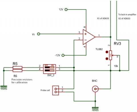
4.2 The admittance to voltage converter
The configuration of the admittance to voltage converter Y/V is a non-inverting operational amplifier (1/2 TL082) as shown in Figure 3.
Figure 3. Circuit of Y/V converter
The voltage at the inverting (-) input will be the same as at the non-inverting (+) input. The sinusoidal voltage $\bar{V}_S$ is then indirectly applied to probe cell whose admittance is $\bar{Y}$. Its current $\bar{I}_S$ flows into resistor RV3.
The output of this stage is the voltage $\bar{V}_Y$ across RV3:
$\bar{V}_Y=R_{V 3} \bar{I}_S$ (12)
where,
$\bar{I}_S=\bar{Y} \bar{V}_S$ (13)
then,
$\bar{V}_Y=R_{V_3} \bar{V}_S \bar{Y}=\bar{K}_Y \bar{Y}$ (14)
where, $\bar{K}_Y$ is the conversion factor given by:
$\bar{K}_Y=R_{V 3} \bar{V}_S$ (15)
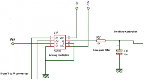
4.3 The phase-sensitive detection
This stage uses a lock-in amplifier to detect the phase θ of admittance $\bar{Y}$ and measure the conductance G from $\bar{V}_Y$. As shown in Figure 4, this stage is composed of analog multiplier and low-pass filter.
Figure 4. Lock-in amplifier circuit based on AD633 multiplier and low-pass filter
The voltage $\bar{V}_Y$ is the complex amplitude of the input vy (between pin1 et pin 2) of AD633 analog multiplier. The $\bar{V}_{S R}$ is the complex amplitude of the reference signal vSR (pin 2 of XR2206) and is applied to pin 3 of AD633. Then,
$v_{S R}=V_{S R} \cos \left(2 \pi f t+\theta_{S R}\right)$ (16)
and
$v_y=V_Y \cos \left(2 \pi f t+\theta_y\right)$ (17)
The output of analog multiplier (pin 6) is the product of two sine waves vSR and vy given by [14]:
$\begin{aligned} & \mathrm{v}_{\mathrm{M}}=K_M \times V_{S R} \cos (2 \pi f t) \times V_Y \cos \left(2 \pi f t+\theta_y\right) \\ & =K_M K_Y V_{S R} \times Y \times \cos (2 \pi f t) \times \cos \left(2 \pi f t+\theta_y\right)\end{aligned}$ (18)
where, KM=0.1 V-1 is the multiplication factor of AD633.
So that,
$v_M=\frac{1}{2} K_M K_Y V_{S R} Y\left[\cos \left(4 \pi f t+\theta_y+\theta_{S R}\right)+\cos \left(\theta_y-\theta_{S R}\right)\right]$ (19)
Since the two inputs vSR and vy of the analog multiplier are at exactly the same frequency, the first term of vM is at frequency of 2f and the second term is a DC voltage given by:
$\mathrm{V}_{\mathrm{G}}=\frac{1}{2} \times K_M K_Y V_{S R} \times Y \times \cos \left(\theta_y-\theta_{S R}\right)$ (20)
The phase θ of admittance $\bar{Y}$ can be determined from Eq. (14), then θy=θSR+θ and VG is given by:
$\mathrm{V}_{\mathrm{G}}=K_M K_Y V_{S R} \times Y \times \frac{1}{2} \times \cos \theta$ (21)
Since the conductance G is defined as the real part of $\bar{Y}$, then,
$\mathrm{G}=Y \times \cos \theta$ (22)
The DC voltage is obtained as:
$\mathrm{V}_{\mathrm{G}}=\frac{1}{2} \times K_M K_Y V_{S R} \times G$ (23)
Using ($\bar{K}_Y=R_{V 3} \bar{V}_S$), the expression of VG can be rewritten as:
$\mathrm{V}_{\mathrm{G}}=K_G \times G$ (24)
where,
$K_G=\frac{1}{2} \times K_M \times R_{V 3} \times V_S \times V_{S R}$ (25)
The first term with frequency 2f is removed using first order passive low-pass filter R7C6. The cutoff frequency is given as:
$f_L=\frac{1}{2 \pi R_7 C_6}$ (26)
4.4 Stage of the microcontroller and LCD
In this stage, the ATMEGA 328P microcontroller is used to read analog signal VG (pin A0) from the follower amplifier (2/2 TL082) connected with the output of low-pass filter R7C6 as shown in Figure 5.
Figure 5. Interfacing circuit measurement with ATMEGA 328P and The LM016L LCD
The analog-to-digital converter (ADC) inside the microcontroller converts this DC voltage to 1024 discrete levels. The potentiometer RV4 is used as a voltage divider to select value of reference voltage in pin REF of ADC.
The values of VG, KM, RV3, VS and VSR are used in the program to calculate value of conductance G. Therefore, electrical conductivity s is calculated from G by using the value of cell constant K trough equations:
$K_G=\frac{1}{2} \times K_M \times R_{V 3} \times V_S \times V_{S R}$ (27)
$G=\frac{V_G}{K_G}$ (28)
$\sigma=K G$ (29)
The pin 5 of double switch DSW in electronic circuit (see Figure 2) is connected with digital input (D4) of microcontroller to select range of electrical conductivity to 1 mS/cm if D4 is at 5 V level and VS at 2 V. If D4 is in 0 V level and VS at 100 mV the range is selected to 20 mS/cm.
The LM016L LCD is used for displaying electrical conductivity. The 4-bit mode is used to send data to LCD and R/W needs to be set to low level. The pin 3 is connected to potentiometer RV5 (10 kΩ) to control the contrast and brightness of the LCD.
Table 1 showed component values for different stages of designed device.
Table 1. Component values of designed device
|
Stage |
Component |
Value |
|
Sinusoidal Voltage Source |
R1 |
200 Ω |
|
R2 |
10 kΩ |
|
|
R3 |
5.1 kΩ |
|
|
R4 |
5.1 kΩ |
|
|
RV1 |
50 kΩ |
|
|
RV2 |
20 kΩ |
|
|
C1 |
100 nF |
|
|
C2 |
1 µF |
|
|
C3 |
10 µF |
|
|
Oscillator |
XR2206 |
|
|
Y/V Converter |
R5 |
100 Ω±0.1% |
|
R6 |
2 kΩ±0.1% |
|
|
RV3 |
10 kΩ |
|
|
Op-Amplifier |
1/2 TL082 |
|
|
Phase-Sensitive Detection |
Multiplier |
AD633 |
|
R7 |
10 kΩ |
|
|
C6 |
10 µF |
|
|
Microcontroller and LCD |
follower amplifier |
2/2 TL082 |
|
Microcontroller |
ATMEGA 328P |
|
|
LCD |
LM016L |
|
|
RV4 |
10 kΩ |
|
|
RV5 |
10 kΩ |
5.1 Setup of the conditioning circuit
According to the specification of XR2206, oscillator temperature stability is optimum for 4 kΩ<R<200 kΩ and 1000 pF<C<100 µF. For this raison the values of R2 and C1 are 10 kΩ and 100 nF respectively and the frequency f is equal to 1 kHz calculated by Eq. (10).
The DC level of output (pin 2) of XR2206 oscillator is suppressed by first order passive high-pass filter RV2 C3. For RV2=20 kΩ and C3=10 µF, the cutoff frequency fH is 0.8 Hz calculated by Eq. (11).
In this device, two ranges to measure electrical conductivity are used. The first is 1 mS/cm and is adjusted by RV1 (50 kΩ) to set VS output (pin 2 of double switched) at 2 V. The second is 20 mS/cm and is adjusted by potentiometer RV2 (20 kΩ) to set VSoutput (pin 2 of double switched) at 100 mV.
The cell conductivity employed in this work has a cell constant K equal to 1 cm-1. As a result, the maximum value of measured conductance is G=1 mS if VS=2 V and G=20 mS if VS=100 mV. For these two cases, the maximum current which flows cell is 2 mA and the RV3 is selected to 5 kΩ to avoid saturation of output of operational amplifier (1/2 TL 082). This maximum output is then at 12 V for 1 mS/cm range and 10.10 V for 1 mS/cm range.
The output of pin 2 of RV2 is used as the reference signal VSR in lock-in amplifier and is adjusted by RV1.The value of VSR is 2 V.
The harmonic with frequency 2f (2 kHz) at output of phase-detection circuit is removed by first order passive low-pass filter R7C6. For R7=10 kΩ and C6=10 µF, the cutoff frequency fL is 1.6 Hz calculated by Eq. (26).
In microcontroller, the potentiometer RV4 (10 kΩ) is used as a voltage divider to set reference voltage (pin REF) of ADC to 1 V which is the maximum of voltage VG for the two ranges.
If the D4 (pin 5 of DSW) is selected at 5 V the value of VS which is used in formula Eq. (27) of KG factor is 2 V and 100 mV if D4 is at 0 V.
5.2 Relative precision of measurement
From Eq. (27), Eq. (28) and Eq. (29) the formula of relative precision of measured electrical conductivity εσ is given by:
$\varepsilon_\sigma=\frac{\Delta \sigma}{\sigma}=\frac{\Delta K}{K}+\frac{\Delta V_G}{V_G}+\frac{\Delta K_M}{K_M}+\frac{\Delta R_{V 3}}{R_{V 3}}+\frac{\Delta V_{S R}}{V_{S R}}+\frac{\Delta V_S}{V_S}$ (30)
A conductivity cell with K=1.0 cm-1 cell constant is the most commonly used because it measures low to high conductivity. Most conductivity cells available on the industry today are delivered with certified cell constants from the manufacturer. The user can simply consider:
$\frac{\Delta K}{K} \approx 0$ (31)
The maximum relative of analog to digital conversion is given by:
$\frac{\Delta V_G}{V_G}=\frac{1}{1024} \approx 0.1 \%$ (32)
The AD633 analog multiplier is laser calibrated to a guaranteed accuracy of 10 V scaling reference and KM multiplication factor KM=1/10 V=0.1 V-1. The maximum value of relative precision of KM is [14]:
$\frac{\Delta K_M}{K_M}=0.25 \%$ (33)
The VSR and VS are measured by digital multimeter with 0.5% maximum relative precision, then:
$\frac{\Delta V_{S R}}{V_{S R}}=\frac{\Delta V_S}{V_S}=0.5 \%$ (34)
So, the maximum relative precision of measured electrical conductivity εσmax can be reduced to
$\varepsilon_{\sigma \max }=\frac{\Delta \sigma \max }{\sigma}= \pm 1.35 \%+\frac{\Delta R_{V 3 \max }}{R_{V 3}}$ (35)
In the case of $\Delta R_{V 3 \max } / R_{V 3}= \pm 0.1 \%$, the value of εσmax is ±1.45%.
5.3 Measurement results
The electronic circuit of designed device can be seen in Figure 6. A 9 V DC battery is connected to SX1308 DC-DC step-up boost converter to provide 12 V DC. The ICL7660 is used to perform conversion from DC positive voltage +12 V to negative voltage -12 V. The voltage regulator 7805 is used to convert +12 V DC to +5 V DC. Theses DC voltages are used to power integrated circuits of fabricated device.
Figure 6. Photos of the designed device for measuring electrical conductivity
According to Eq. (35), the precision multiturn potentiometer RV3= 10 kΩ was used and adjusted at 5 kΩ to achieve the minimum of εσ and to calibrate the device in two ranges 20 mS/cm and 1 mS/cm by using commercial standard solutions (74.0 µS/cm±0.7% and 1.406 mS/cm±0.5%).
Standard solutions are susceptible to contamination from atmospheric carbon dioxide and thus increasing the conductivity. To overcome this problem, the precision resistors (R5=100 Ω ±0.1% and R6=2 kΩ ±0.1%) are employed instead of probe cell (see Figure 3.) to simulate conductive solutions (10 mS/cm±0.1% and 500 µS/cm±0.1%).
To check the reproducibility and accuracy of measurements and the effectiveness of phase sensitive detection, a combination of resistors RS and capacitor CS was used to simulate conductive solutions/capacitive influence in probe cell.
Table 2. Conductivity measurement results of simulated solutions
|
RS |
CS |
σM |
GM |
GS |
εMS |
|
100 Ω ±1% |
1 µF |
10.04 mS/cm |
10.04 mS |
10 mS ±1% |
0.4% |
|
100 nF |
10.04 mS/cm |
10.04 mS |
10 mS ±1% |
0.4% |
|
|
10 nF |
10.04 mS/cm |
10.04 mS |
10 mS ±1% |
0.4% |
|
|
10 kΩ ±1% |
1 µF |
100.6 µS/cm |
100.6 µS |
100 µS ±1% |
0.6% |
|
100 nF |
100.6 µS/cm |
100.6 µS |
100 µS ±1% |
0.6% |
|
|
10 nF |
100.6 µS/cm |
100.6 µS |
100 µS ±1% |
0.6% |
|
|
100 kΩ ±1% |
1 µF |
9.93 µS/cm |
9.93 µS |
10 µS ±1% |
0.7% |
|
100 nF |
9.93 µS/cm |
9.93 µS |
10 µS ±1% |
0.7% |
|
|
10 nF |
9.93 µS/cm |
9.93 µS |
10 µS ±1% |
0.7% |
Table 2 showed conductivity measurements σM for different values of RSCS where GS is the conductance that is reciprocal of RS and GM is conductance corresponding to measured conductivity σM with GM=sM/K and K=1.
The impedances of capacitors CS: 1µF, 100 nF and 10 nF which simulated conductive solutions/capacitive influence at f=1 kHz respectively correspond to 160 Ω, 1.60 kΩ and 16 kΩ.
As can be seen in Table 2, the measured conductivity values are directly related to simulation resistance value and are independent of the capacitance values.
These results confirm that the fabricated device only measures the electrical conductivity without the capacitive influence in probe cell.
From Table 2, the maximum value of relative difference εMS between GS and GM for different values of RS and CS was 0.7% which is less than the value of tolerance of RS.
The fabricated device has been used to measure conductivities of the NaCl, KCl, CaCl2, MgSO4 for different concentrations maintained at 25℃.
Table 3. Measurement results of different solutions
|
Solution |
σF |
σC |
εFC % |
|
NaCl 9 g/L |
17.90 mS/cm |
18.36 mS/cm |
2.57 |
|
NaCl 4.5 g/L |
12 mS/cm |
9.21 mS/cm |
2.68 |
|
KCl 10 g/L |
12.81 mS/cm |
13.16 mS/cm |
2.73 |
|
KCl 5 g/L |
7.20 mS/cm |
7.39 mS/cm |
2.64 |
|
CaCl2 10 g/L |
9.114 mS/cm |
9.351 mS/cm |
2.60 |
|
CaCl2 10 g/L |
4.974 mS/cm |
5.102 mS/cm |
2.57 |
|
MgSO4 15 g/L |
6.39 mS/cm |
6.57 mS/cm |
2.82 |
|
MgSO4 7.5 g/L |
3.754 mS/cm |
3.836 mS/cm |
2.18 |
Table 3 showed conductivity measurement results that are compared with those measured by commercial conductivity meter (Shengmeiyu TDS&EC).
From Table 3, the minimum and maximum relative differences εFC of conductivity measurements between fabricated device σF and commercial conductivity meter σC were respectively 2.18% and 2.82%.
Figure 7. Calibration curve for concentration of NaCl
The concentrations of electrolyte solutions can be determined by measuring conductivity of the solution [15-18]. The example of calibration curve obtained by fabricated device is shown in Figure 7 corresponding to NaCl solution.
The equation of calibration is given by:
$\sigma_M=K_C C+\sigma_{M 0}$ (36)
where,
C is the concentration of solution, mg/L;
σM is measured conductivity, mS/cm;
KC=0.0020 mS.L.mg-1.cm-1 is the calibration constant;
σM0=0.0796 mS/cm is the initial conductivity.
This equation is obtained by least square curve fitting. The mean relative error was 1.32% and the coefficient of determination was 0.9998.
The device has also been used to measure conductivities of the hemodialysis solutions, for which the values of conductivities are known [19-21].
Table 4 showed conductivity measurement results that are compared with those measured by commercial conductivity meter (Shengmeiyu TDS&EC).
Table 4. Measurement results of different solutions
|
Solution |
σF |
σC |
εFC % |
|
Carbon filter |
1.021 mS/cm |
1.048 mS/cm |
2.64 |
|
Water softener |
841 µS/cm |
857 µS/cm |
1.90 |
|
Reverse osmosis |
67.00 µS/cm |
68.57 µS/cm |
2.34 |
|
Dialysate |
14.60 mS/cm |
14.90 mS/cm |
2.05 |
The ISO23500 standard recommends daily measuring of conductivity both pre- and post -filtration and percentage efficiency in the water reverse osmosis unit. Conductivity of dialysate should be checked with calibrated measuring device. Conductivity measurement ensures proper water-to-concentrate ratio of the dialysate [22, 23].
From Table 4, the minimum and maximum relative difference εFC of conductivity measurements between fabricated device σF and commercial conductivity meter σC were respectively 1.90% and 2.64%.
The purpose of this work is to measure electrical conductivity by using a phase sensitive detection technique and an admittance to voltage converter to eliminate problem of equilibrium conditions in bridge technique which cannot provide a rapid measurement of conductivity. The other most important advantage of this technique is that it provides value of conductance and eliminates capacitive influence in probe cell/solution admittance. It also has the advantages of low cost, simple design compared to Fourier analysis of complex admittance.
The design of conditioning circuit is based on XR2206 sinusoidal generator source, an admittance to voltage converter realized by non-inverting amplifier, a lock-in amplifier realized by AD633 multiplier and RC filter, an ATMEGA 328P microcontroller card. The conductivity of solution is displayed on The LM016L LCD after processing by microcontroller.
The high accuracy of proposed conductivity meter is related to the high relative precision of values of KM, RV3, VS, VSR, VG and K.
The experimental results show that design of this device is successful. The level of agreement between values of simulated conductive solutions with tolerance 1% and measured conductivity (maximum is 0.7%) is satisfactory to confirm the measurement accuracy of the developed device.
The effective calibration can be performed by 0.1% precision resistors and maximum value of relative error of measured conductivity is 1.45% which is lower than that of commercial conductivity meters (generally 2%; see for example technical specifications of Elcometer, Extech, Runge or Hanna conductivity meters).
To verify compliance with IEC61326 EMC/IEC60610 safety standards, the device should pass the EMC/safety tests approved by ISO 17025 accredited laboratories. In accordance with IEC61010 standard, the measuring category of this device is CAT I because it is used to measure the conductivity of solutions without connection to the mains which cannot be allocated to categories CAT II and CAT IV. The class of electrical safety is III because the input voltage is 9 V DC and is not at a hazardous level and thus the user does not need to be protected from this input voltage.
The performance of fabricated device can be improved by auto range selection based on analog multiplexers and voltage dividers connected to the output of oscillator. In order to miniaturize the device, the sinewave of oscillator can be generated by using Pulse Width Modulation PWM in microcontroller and active low-passe filter.
Finally, the 20 mS/cm and 1 mS/cm measurement ranges are most suitable for industrial and biomedical applications such as assuring water quality based upon ISO standards and facilitating maintenance by biomedical engineers in center hemodialysis.
We would like to express our sincere gratitude to the University Hospital Center of Tlemcen for supporting this work and providing electrolytes solutions.
[1] Silný, A., Haugsdal, B. (1993). Electrical conductivity measurements of corrosive liquids at high temperatures. Review of Scientific Instruments, 64(2): 532-537. https://doi.org/10.1063/1.1144228
[2] Schiefelbein, L., Fried, A., Rhoads, G., Sadoway, R. (1998). A high-accuracy, calibration-free technique for measuring the electrical conductivity of liquids. Review of Scientific Instruments, 69(9): 3308-3313. https://doi.org/10.1063/1.1149095
[3] García-Breijo, E., Barat, M., Torres, L., Grau, R., Gil, L., Ibánez, J., Alcaniz, M., Masto, R., Fraile, R. (2008). Development of a puncture electronic device for electrical conductivity measurements throughout meat salting. Sensors and Actuators A: Physical, 148(1): 63-67. https://doi.org/10.1016/j.sna.2008.07.013
[4] Yudhana, A., Septiyani, R., Mufandi, I., Rosyady, P., Husein, M., Abdullatif. L. (2022). A portable device based on an electrical conductivity sensor for the detection of monosodium glutamate (MSG) in soupy foods. Instrumentation Mesure Métrologie, 21(3): 119-126. https://doi.org/10.18280/i2m.210305
[5] Sophocleous, M., Atkinson, J., Smethurst, J., Espindola-Garcia, G., Ingenito, A. (2020). The use of novel thick-film sensors in the estimation of soil structural changes through the correlation of soil electrical conductivity and soil water content. Sensors and Actuators A: Physical, 301(1): 1-7. https://doi.org/10.1016/j.sna.2019.111773
[6] Ravagli, E., Crescentini, M., Tartagni, M., Severi, S. (2017). Non-invasive measurement of electrical conductivity of liquids in bio-compatible polymeric lines for hemodialysis applications. Sensors and Actuators A: Physical, 261(1): 251-260. https://doi.org/10.1016/j.sna.2017.04.034
[7] Munoz, D., Berga, S. (2005). An analog electronic interface to measure electrical conductivity in liquids. Measurement, 38(3): 181-187. https://doi.org/10.1016/j.measurement.2005.07.013
[8] Rajendran, A., Neelamegam, P. (2004). Measurement of conductivity of liquids using AT89C55WD microcontroller. Measurement, 35(1): 59-63. https://doi.org/10.1016/j.measurement.2003.08.015
[9] Oliver, B., Cage, M., (1971). Electronic measurement and instrumentation. McGraw-Hill, New York.
[10] Marioli, D., Sardini, E., Taroni, A. (1993). High accuracy measurement technique for capacitive transducers. Measurement Science and Technology, 4(3): 337-343. https://doi.org/10.1088/0957-0233/4/3/012
[11] Takagishi, E. (1980). On the balance of an AC wheatstone bridge. IEEE Transactions on Instrumentation and Measurement, 29(2): 131-136. https://doi.org/10.1109/Tim.1980.4314886
[12] Javier Lario-Garcıa, J., Pallas-Areny, R. (2006). Constant-phase element identification in conductivity sensors using a single square wave. Sensors and Actuators A: Physical, 132(1): 122-128. https://doi.org/10.1016/j.sna.2006.04.014
[13] XR2206 Datasheet (2008). Exar corporation. https://www.alldatasheet.com/datasheet-pdf/pdf/80496/EXAR/XR2206.html.
[14] Low-cost analog multiplier AD633, datasheet, https://www.analog.com/media/en/technical-documentation/data-sheets/ad633.pdf.
[15] Quan, X., Fu, Z., Yuan, L., Zhong, M., Mi, R., Yang, X., Yi. Y., Xang, C. (2017). Capacitive deionization of NaCl solutions with ambient pressure dried carbon aerogel microsphere electrodes. RSC Advances, 7(1): 5875–35882. https://doi.org/10.1039/C7RA05226J
[16] Tong, J., Yang, J., Hu, B., Sun, H. (2016). Experimental study on soluble chemical transfer to surface runoff from soil. Environmental Science and Pollution Research, 23(20): 20378–20387. https://doi.org/10.1007/s11356-016-7248-2
[17] Tadimeti, J., Jain, S., Chattopadhyay, S., Bhattacharya P. (2014). Selection of the best process stream to remove Ca2+ ion using electrodialysis from sugar solution. International Journal of Electrochemistry, 2014(1): 1-12. https://doi.org/10.1155/2014/304296
[18] Tomsic, T., Marija, B., Jamnik, A. (2002). Conductivity of magnesium sulfate in water from 5 to 35° and from infinite dilution to saturation. Journal of Solution Chemistry, 31(1): 19-31. https://doi.org/10.1023/A:1014853001357
[19] Suhail, A. (2005). Essentials of water treatment in hemodialysis. Hemodialysis International, 9(2): 127-134. https://doi.org/10.1111/j.1492-7535.2005.01124.x
[20] Dheda, S., Van Eps, C., Hawley, C., Johnson, D.W. (2015). Water treatment for center and home-based hemodialysis. Updates in Hemodialysis. https://doi.org/10.5772/59380
[21] Bertinsson, G. (2012). The conductivity of dialysis fluid. Journal of Renal Care, 31(1): 31-34. https://doi.org/10.1111/j.1755-6686.2005.tb00387.x
[22] International Organization for Standardization. (2019). ISO 23500-5:2019 Quality of dialysis fluid for haemodialysis and related therapies (No. ISO 23500-5:2019). https://www.iso.org/standard/67614.html.
[23] International Organization for Standardization. (2019). ISO 23500-2:2019 Water treatment equipment for haemodialysis applications and related therapies (No. ISO 23500-2:2019). https://www.iso.org/standard/67611.html.