Funmilayo H. Oyelami* | Ebenezer O. Ige | Olaide Y. Saka-Balogun | Oluwaseyi A. Adeyemo
© 2021 IIETA. This article is published by IIETA and is licensed under the CC BY 4.0 license (http://creativecommons.org/licenses/by/4.0/).
OPEN ACCESS
This numerical investigation reports the unsteady MHD pulsatile flow of couple stress Non-Newtonian fluid. In the fluid, the effect of non-uniform wall temperature and concentration as a result of periodic heat and mass input at the heated wall was taken into consideration. Also, the influence of a uniform external magnetic field between two parallel plates was considered. The pressure driven fluid was analysed using Eyring-Powell Non-Newtonian fluid model. The non-linear dimensional partial differential equations, under some assumptions, are transformed into a set of dimensionless equations. The solution to the dimensionless equations is obtained using spectral relaxation techniques (SRM). Graphical results are provided for different values of fluid parameters.
heat and mass transfer, couple stress, MHD, pulsatile, spectral relaxation method
Study of Oscillatory fluid have several applications in pulsatile blood flow through the arteries, movement of fluid in the intestine, etcetera. Research on Non-Newtonian fluid is gradually finding its way towards that direction due to the failure of Newtonian model to predict the rheological behaviour of complex fluids. Over the years, there have been many models to study the behaviour of many non-Newtonian fluids. One of these is the Eyring-Powell model.
Investigations of transient MHD Non-Newtonian fluid flow has been established for fluids involving zero-acceptance approximation and for planar porous walls. MHD fluid flows needs more time to acquire uniform velocity distribution.
Couple stress is the consequence of the assumption that mechanical action of one part of a body on another across a surface is equivalent to a force and moment distribution. The noticeable feature of couple stress fluid is the addition of the size dependent effect that is generally disregarded in the established continuum mechanics.
Several works have been done on the transfer of heat to fluid flow having the effect of couple stress using Eyring-Powell rheological model. Some of these studies include Adesanya et al. [1] in their investigation on the heat transfer to the transient pulsatile hydromagnetic flow under couple stresses through porous channel. Effect of couple stresses on the MHD of a non-Newtonian unsteady flow between two parallel porous plates was considered by Eldabe et al. [2]. The incompressible couple stress flow of fluid between parallel disks was considered by Srinivasacharya and Kaladhar [3].
Using Adomian decomposition approach and Eyring-Powell non-Newtonian fluid model, existence and uniqueness of the solution to the pulsatile couple stress was proved by Adesanya and Ayeni [4]. Adesanya and Makinde [5] investigated the heat transfer to magnetohydrodynamic non-Newtonian couple stress pulsatile flow between two parallel porous plates using Eyring-Powell model. Using network numerical simulation, Zueco and B’eg [6] studied pulsatile non-Newtonian flow through a channel having the effects of couple stress and wall mass flux.
In recent years, colossal accomplishments have been made on the radiative heat transfer to flow of oscillatory flows and different mathematical descriptions of these flows have been developed by several authors. Some of the study include Tsai and Hsu [7], who applied meshless numerical approach to investigate oscillatory Stokes flows in convection and convective flows in porous media by using the method of fundamental solutions. Zakaria [8] studied the effects of free convection currents on the oscillatory flow of a viscoelastic fluid with thermal relaxation in the presence of a transverse magnetic field bounded by a vertical plane surface. Effects of radiative heat transfer and magnetohydrodynamics on an oscillatory flow in a channel filled with a porous medium using an analytical approach is considered by Makinde and Mhone [9]. For a two-dimensional oscillatory flow, Hakeem and Sathiyanathan [10] studied analytical solutions on free convective radiation of an incompressible viscous fluid through a highly porous medium bounded by an infinite vertical plate. Mahmoud and Ali [11] examined an unsteady oscillatory flow of an incompressible viscous fluid in a planar channel filled with a porous medium in the presence of a transverse magnetic field.
In all the above studies, the combined effects of heat and mass transfer to the fluid flow was not given attention. Whereas, several industrial processes which includes cooling of nuclear reactors, plasma studies and petroleum industries involve flows that occur at a very high temperature and concentration which makes the effect of thermal radiation and chemical reaction very important for enhanced cooling of the system.
The purpose of this paper is to examine the effect of radiative heat and mass transfer on magnetohydrodynamic non-Newtonian couple stress fluid flow through parallel porous plates with non-uniform wall temperature and concentration using the Erying–Powel rheological model, which has not been considered in literature. To achieve this, the governing boundary layer equations were transformed into a non-dimensional form and the dimensionless equations together with the boundary conditions are solved using spectral relaxation techniques (SRM). To apply this method, iterations at the current level is assumed to be evaluated at (r+1) while other terms such as linear and nonlinear are assumed to be known at the previous iteration denoted by (r). The method has been applied to different mathematical problems some of which are carried out by Idowu and Falodun [12], Alao et. al [13].
Consider a non-Newtonian transient incompressible, electrically conducting fluid between two parallel porous plates at distance $h$ apart under the influence of couple stress and externally applied magnetic field. The $x-$ axis lies along the centre of the channel while the $y-$ axis represent the distance measured normal to it. The fluid is injected into the lower wall at $y=0$ and absorbed in with the same constant velocity $V_{0}$ through the upper wall at $y=l$. Assuming all fluid properties are constant with small electrical conductivity except that of fluid density that varies with temperature and the electromagnetic force produced is very small. The governing equations, assuming Boussinesq incompressible fluid model are given as
$\frac{\partial u^{*}}{\partial t^{*}}+V_{0} \frac{\partial u^{*}}{\partial y^{*}}=-\frac{1}{\rho} \frac{\partial P^{*}}{\partial x^{*}}+\frac{1}{\rho} \frac{\partial}{\partial y^{*}}\left(\tau_{x y}\right)-\frac{\sigma B_{0}^{2} u^{*}}{\rho}-\frac{\eta}{\rho} \frac{\partial^{4} u^{*}}{\partial y^{* 4}}+$$\mathrm{g} \beta_{T}\left(T^{*}-T_{0}^{*}\right)+g \beta_{c}\left(C^{*}-C_{0}^{*}\right)$ (1)
$\frac{\partial T^{*}}{\partial t^{*}}+V_{0} \frac{\partial T^{*}}{\partial y^{*}}=\frac{k}{\rho C_{p}} \frac{\partial^{2} T^{*}}{\partial y^{*2}}-\frac{1}{\rho C_{p}} \frac{\partial q_{r}}{\partial y^{*}}$ (2)
$\frac{\partial C^{*}}{\partial t^{*}}+V_{0} \frac{\partial C^{*}}{\partial y^{*}}=D \frac{\partial^{2} C^{*}}{\partial y^{*^{2}}}$ (3)
with the following boundary conditions
$u^{*}=0, \frac{\partial^{2} u^{*}}{\partial y^{* 2}}=0, T^{*}=T_{0}, C^{*}=C_{0} \quad$ at $y^{*}=0$ (4)
$u^{*}=0, \frac{\partial^{2} u^{*}}{\partial y^{* 2}}=0, T^{*}=T_{1}+\left(T_{1}-T_{0}\right) \cos \omega t, C^{*}$$=C_{1}+\left(C_{1}-C_{0}\right) \cos \omega t$ at $y^{*}$$=l$ (5)
where, $u^{*}$ is the velocity, $t^{*}$ the time, $P^{*}$ is the pressure, $T^{*}$ the fluid temperature, $C^{*}$ the fluid concentration, $\rho$ is the fluid density, $\tau_{x y}$ the stress tensor, $\sigma$ the conductivity of the fluid, $B_{0}$ the electromagnetic induction, $\eta$ the couple stress parameter, $V_{0}$ the suction/injection parameter, $g$ the gravitational force, $\beta_{C}$ the coefficient of volume expansion due to concentration, $\beta_{T}$ the coefficient of volume expansion due to temperature, $D$ is the chemical molecular diffusivity,$C_{p}$ the specific heat at constant pressure, $k$ the thermal conductivity and $q_{r}$ the radiative heat flux.
For fluid in optically thin limit, there is no self-absorption, but rather, fluid only absorbs radiations from the boundaries. The radiative heat flux in the energy equation, approximated in the optically thin limit according to Oyelami and Dada [14] is given as
$\frac{\partial q_{r}}{\partial y^{*}}=4\left(T^{*}-T_{0}^{*}\right) L$ (6)
where, L is the mean absorption coefficient.
Also, the stress tensor for Eyring-Powell visco-elastic model is modified according to Oyelami and Dada [14] as follows:
$T_{x y}=\mu \frac{\partial u^{*}}{\partial y^{*}}+\frac{1}{\alpha} \sinh ^{-1}\left(\frac{1}{c} \frac{\partial u^{*}}{\partial y^{*}}\right)$ (7)
where, $\mu$ is the coefficient of dynamic viscosity, $\alpha$ and $c$ characterizes the Eyring-Powell fluid model.
The expansion of the elastic part in Eq. (6), neglecting higher-order terms gives
$\sin h^{-1}\left(\frac{1}{c} \frac{\partial u^{*}}{\partial y^{*}}\right) \cong \frac{1}{c} \frac{\partial u^{*}}{\partial y^{*}}+O(.)^{3},\left|\frac{1}{c} \frac{\partial u^{*}}{\partial y^{*}}\right|<1$ (8)
Hence the stress tensor for Eyring-Powell model becomes
$T_{x y}=\mu \frac{\partial u^{*}}{\partial y^{*}}+\frac{1}{\alpha c} \frac{\partial u^{*}}{\partial y^{*}}$ (9)
The following dimensionless parameters and variables are introduced
$X=\frac{x^{*}}{l}, Y=\frac{y^{*}}{l}, U=\frac{u^{*}}{V_{0}}, t=\frac{t^{*} V_{0}}{l}, P=\frac{P^{*}}{\rho V_{0}^{2}}, T=$$\frac{T^{*}-T_{0}^{*}}{T_{w}^{*}-T_{0}^{*}}, C=\frac{C^{*}-C_{0}^{*}}{C_{w}^{*}-C_{0}^{*}}, R e=\frac{l V_{0}}{v}, S c=\frac{V_{0} l}{D}$
$N=\frac{4 L}{\rho C p V_{0}}, P e=\frac{\rho C p V_{0} l}{k}, G r=\frac{g \beta_{T}\left(T_{w}^{*}-T_{0}^{*}\right)}{v V_{0}}, G m=$$\frac{g \beta_{C}\left(C_{w}^{*}-C_{0}^{*}\right) h^{2}}{v V_{0}} H^{2}=\frac{\sigma B_{0}^{2} l^{2}}{\mu}, \mathrm{M}=\frac{1}{\alpha \mu c}$ (10)
where, $a^{2}$ is the inverse of the couple stress parameter, $P e$ is the Peclet number, $H^{2}$ is the Hartmann number, $M$ is the Eyring-Powell parameter, $G m$ the Grashof number, $G c$ is the modified Grashof number, $R e$ is the Reynolds number, $l$ is the characteristic length of the channel, $T$ is the dimensionless temperature, $C$ is the dimensionless concentration and $N$ is the thermal radiation parameter.
Applying Eqns. (5), (8) and (9) in (1), (2) and (4), we obtain the following dimensionless equations
$\frac{\partial U}{\partial t}+\frac{\partial U}{\partial Y}=-\frac{\partial P}{\partial X}+\frac{(1+M)}{R e} \frac{\partial^{2} U}{\partial Y^{2}}-\frac{H^{2}}{R e} U-\frac{1}{a^{2} R e} \frac{\partial^{4} U}{\partial Y^{4}}$$+G r T+G m C$ (11)
$\frac{\partial T}{\partial t}+\frac{\partial T}{\partial Y}=\frac{1}{P e} \frac{\partial^{2} T}{\partial Y^{2}}-N T$ (12)
$\frac{\partial C}{\partial t}+\frac{\partial C}{\partial Y}=\frac{1}{S c} \frac{\partial^{2} C}{\partial Y^{2}}$ (13)
With these dimensionless boundary conditions
$U=0, \frac{\partial^{2} U}{\partial Y^{2}}=0, T=0, C=0$ at $Y=0$ (14)
$U=0, \frac{\partial^{2} U}{\partial Y^{2}}=0, T=1+\cos \omega t, C=1+\cos \omega t$ at $Y=1$ (15)
This section gives detailed explanation of an iterative method called spectral relaxation techniques (SRM). To apply this method, iterations at the current level is assumed to be evaluated at $(r+1)$ while other terms such as linear and nonlinear are assumed to be known at the previous iteration denoted by $(r)$. The above description on SRM is in line with the idea of Gauss-seidel of decoupling linear system of equation. This work uses the Chebyshev spectral collocation methods to discretize the differential equations. To apply the spectral methods, the domain on which the governing equation is defined is transformed to the interval $[-1,1]$. It is on this transformed domain that the spectral method can be implemented. The transformation $\eta=\frac{L(\tau+1)}{2}$ is used to map the interval $[0, L]$ to $[-1,1]$ where $L$ is the scalling parameter approximated its conditions at infinity. As a result of the SRM scheme procedure described above, equations (11)-(13) becomes
$\frac{\partial u_{r+1}}{\partial t}=a_{0, r} \frac{\partial^{2} u_{r+1}}{\partial Y^{2}}-\frac{\partial u_{r+1}}{\partial Y}+a_{r+1} \frac{\partial^{4} u_{r+1}}{\partial Y^{4}}$$-\frac{H^{2}}{R e} u_{r+1}+a_{2, r}$ (16)
$\frac{\partial T_{r+1}}{\partial t}=b_{0, r} \frac{\partial^{2} T_{r+1}}{\partial Y^{2}}-\frac{\partial T_{r+1}}{\partial Y}-N T_{r+1}$ (17)
$\frac{\partial C_{r+1}}{\partial t}=c_{0, r} \frac{\partial^{2} C_{r+1}}{\partial Y^{2}}-\frac{\partial C_{r+1}}{\partial Y}$ (18)
Subject to the boundary conditions
$u_{r+1}(0, t)=0, \quad u_{r+1}^{\prime \prime}(0, t)=0 T_{r+1}=0$, $C_{r+1}=0$ (19)
$u_{r+1}(l, t)=0, \quad u_{r+1}^{\prime \prime}(l, t)=0$,
$T_{r+1}(l, t)=1+\cos (\omega t)$, $C_{r+1}(l, t)=1+\cos (\omega t)$ (20)
The basic concept of spectral collocation method is the introduction of Chebyshev differentiation matrix D. It is used to approximate the derivatives of the unknown variables at the points of collocation matrix vector product of the form
$\frac{d u_{r}}{d y}=\sum_{k=0}^{N} D_{i k} u_{r}\left(\tau_{k}\right)=D u_{r}, \quad i=0,1, \ldots, N$ (21)
$\frac{d T_{r}}{d y}=\sum_{k=0}^{N} D_{i k} T_{r}\left(\tau_{k}\right)=D T_{r}, \quad i=0,1, \ldots, N$ (22)
$\frac{d C_{r}}{d y}=\sum_{k=0}^{N} D_{i k} C_{r}\left(\tau_{k}\right)=D C_{r}, \quad i=0,1, \ldots, N$ (23)
where, $N+1$ is the number of grid points $D=\frac{2 D}{\eta}$ and $u=$ $\left[u\left(Y_{0}\right), u\left(Y_{1}\right), \ldots, u\left(Y_{N x}\right)\right]^{T}, T=\left[T\left(Y_{0}\right), T\left(Y_{1}\right), \ldots, T\left(Y_{N x}\right)\right]^{T}$ and $C=\left[C\left(Y_{0}\right), C\left(Y_{1}\right), \ldots, C\left(Y_{N x}\right)\right]^{T} .$
The initial approximation for solving (11)-(13) with due consideration of the boundary conditions (14) and (15) when y=0 is given as
$u_{0}=(y, t)=1-e^{-y}$, $T_{0}(y, t)=e^{-y}+\cos (\omega t)$, $C_{0}(y, t)=e^{-y}+\cos (\omega t)$ (24)
Starting from the above initial approximations (24), the schemes in equations (16)-(18) subject to (19) and (20) can be solved iteratively for $u_{r+1}(y, t), T_{r+1}(y, t)$ and $\mathrm{C}_{r+1}(y, t)$ when $r=0,1,2, \ldots$ Following Motsa et al.[?], the GaussLobatto collocation points is used to define the nodes in $[-1,1]$ as
$Y_{j}=\cos \left(\frac{\pi j}{N x}\right), \quad j=0,1, \ldots, N x$ (25)
The finite difference method with centering about a midpoint between $t^{n+1}$ and $t^{n}$ is applied on the iteration schemes $(16)-(18)$. The centering about $t^{n+\frac{1}{2}}$ to any of the unknown function, say $u(y, t)$ and its associated derivative leads to
$u\left(y_{j}, t^{n+\frac{1}{2}}\right)=u_{j}^{n+\frac{1}{2}}=\frac{u_{j}^{n+1}+u_{j}^{n}}{2}$,$\left(\frac{\partial u}{\partial t}\right)^{n+\frac{1}{2}}=\frac{u_{j}^{n+1}-u_{j}^{n}}{\Delta t}$ (26)
$T\left(y_{j}, t^{n+\frac{1}{2}}\right)=T_{j}^{n+\frac{1}{2}}=\frac{T_{j}^{n+1}+T_{j}^{n}}{2}$,$\left(\frac{\partial T}{\partial t}\right)^{n+\frac{1}{2}}=\frac{T_{j}^{n+1}-T_{j}^{n}}{\Delta t}$ (27)
$C\left(y_{j}, t^{n+\frac{1}{2}}\right)=C_{j}^{n+\frac{1}{2}}=\frac{\mathrm{C}_{j}^{n+1}+\mathrm{C}_{j}^{n}}{2}$, $\left(\frac{\partial C}{\partial t}\right)^{n+\frac{1}{2}}=\frac{C_{j}^{n+1}-C_{j}^{n}}{\Delta t}$ (28)
The spectral method is first applied on (16)-(18) before applying the finite difference method to give
$\frac{d u_{r+1}}{d t}=\left(a_{0, r} D^{2}-D+a_{1, r} D^{4}-\frac{H^{2}}{R e}\right) u_{r+1}+a_{2, r}$ (29)
$\frac{d T_{r+1}}{d t}=\left(b_{0, r} D^{2}-D-N\right) T_{r+1}$ (30)
$\frac{d C_{r+1}}{d t}=\left(c_{0, r} D^{2}-D\right) C_{r+1}$ (31)
subject to (19) and (20) where
$u_{r+1}=\left[\begin{array}{l}u_{r+1}\left(x_{0}, t\right) \\ u_{r+1}\left(x_{1}, t\right) \\ \vdots \\ u_{r+1}\left(x_{N_{x-1}}, t\right) \\ u_{r+1}\left(x_{N_{x}}, t\right)\end{array}\right]$, $T_{r+1}=\left[\begin{array}{l}T_{r+1}\left(x_{0}, t\right) \\ T_{r+1}\left(x_{1}, t\right) \\ \vdots \\ T_{r+1}\left(x_{N_{x-1}}, t\right) \\ T_{r+1}\left(x_{N_{x}}, t\right)\end{array}\right]$, $C_{r+1}=\left[\begin{array}{l}C_{r+1}\left(x_{0}, t\right) \\ C_{r+1}\left(x_{1}, t\right) \\ \vdots \\ C_{r+1}\left(x_{N_{x-1}}, t\right) \\ C_{r+1}\left(x_{N_{x}}, t\right)\end{array}\right]$ (32)
$a_{0, r}=\left[\begin{array}{lllll}a_{0, r}\left(x_{0}, t\right) & & \\ & a_{0, r}\left(x_{1}, t\right) & & & \\ & & \ddots & & \\ & & & \ddots & \\ & & & & a_{0, r}\left(x_{N_{x}}, t\right)\end{array}\right]$
$a_{1, r}=\left[\begin{array}{lllll}a_{1, r}\left(x_{0}, t\right) & & \\ & a_{1, r}\left(x_{1}, t\right) & & & \\ & & \ddots & & \\ & & & \ddots & \\ & & & & a_{1, r}\left(x_{N_{x}}, t\right)\end{array}\right]$
$b_{0, r}=\left[\begin{array}{lllll}b_{0, r}\left(x_{1}, t\right) & & \\ & b_{0, r}\left(x_{2}, t\right) & & & \\ & & \ddots & & \\ & & & \ddots & \\ & & & & b_{0, r}\left(x_{N_{x}}, t\right)\end{array}\right]$
$c_{0, r}=\left[\begin{array}{lllll}c_{0, r}\left(x_{1}, t\right) & & \\ & c_{0, r}\left(x_{2}, t\right) & & & \\ & & \ddots & & \\ & & & \ddots & \\ & & & & c_{0, r}\left(x_{N_{x}}, t\right)\end{array}\right]$ (33)
We now proceed to apply the finite difference scheme on Eqns. (29)-(31) in the $t-$ direction with the mid-point $t^{n+\frac{1}{2}}$ to yield
$A_{1} u_{r+1}^{n+1}=A_{2} u_{r+1}^{n}+K_{1}$ (34)
$B_{1} T_{r+1}^{n+1}=B_{2} T_{r+1}^{n}+K_{2}$ (35)
$M_{1} C_{r+1}^{n+1}=M_{2} C_{r+1}^{n}+K_{3}$ (36)
Subject to the boundary conditions
$u_{r+1}\left(x N x, t^{n}\right)=T_{r+1}\left(x N x, t^{n}\right)=C_{r+1}\left(x N x, t^{n}\right)=0$ (37)
$u_{r+1}\left(x_{0}, t^{n}\right)=0, \quad u_{r+1}^{\prime \prime}\left(x_{0}, t^{n}\right)$$=0 T_{r+1}\left(x_{0}, t^{n}\right)=1+\cos (\omega t)$, $C_{r+1}\left(x_{0}, t^{n}\right)=1+\cos (\omega t)$ (38)
where
$A_{1}=\frac{1}{\delta t}-\frac{1}{2}\left(a_{0, r} D^{2}-D+a_{1, r} D^{4}-\frac{H^{2}}{R e}\right)$,
$A_{2}=\frac{1}{\delta t}+\frac{1}{2}\left(a_{0, r} D^{2}-D+a_{1, r} D^{4}-\frac{H^{2}}{R e}\right)$,
$B_{1}=\frac{1}{\delta t}-\frac{1}{2}\left(b_{0, r} D^{2}-D-N\right)$, $B_{2}=\frac{1}{\delta t}+\frac{1}{2}\left(b_{0, r} D^{2}-D-N\right)$,
$M_{1}=\frac{1}{\delta t}-\frac{c_{0, r} D^{2}-D}{2}$, $M_{2}=\frac{1}{\delta t}+\frac{c_{0, r} D^{2}-D}{2}$,
$K_{1}=a_{2, r}^{n+1}, \quad K_{2}=I, \quad K_{3}=I$
An efficient method called spectral relaxation method (SRM) has been used to solve the transformed Eqns. (11)-(13) along with the boundary conditions (14) and (15) numerically. The present paper examined the effect of pertinent flow parameters on the velocity, temperature and concentration profiles.
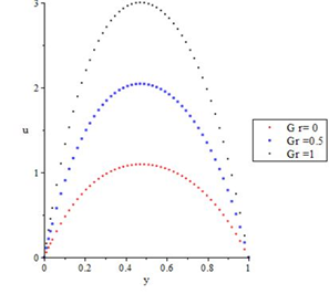
Figure 1 represents the effect of the thermal Grashof number on the velocity profile. Obviously from the Figure 1, when Gr=0, the flow attains minimum value and as it increases the flow attains maximum value. Physically, the thermal buoyancy force gives rise to buoyancy force which enhances the hydrodynamics within the boundary layer. The result in Figure 1 implies that the buoyancy force has a great significant effect on the flow.
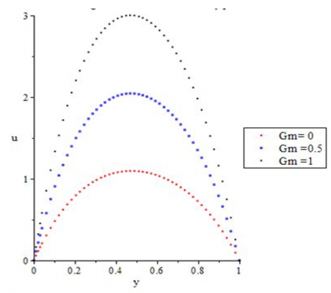
The effect of an increase in the mass Grashof number is represented in Figure 2. The result shows that increase in mass buoyancy enhances the concentration effects.
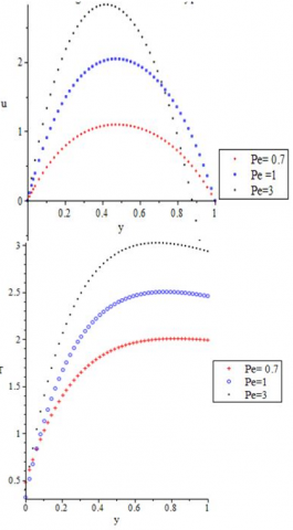
Figure 3 shows the effect of Peclet number on the velocity and temperature profiles. Increasing Peclet number is seen to bring increase to both velocity and temperature profile. Peclet number represents the ratio of heat transfer by fluid motion to the one by thermal conduction. Increase in the fluid thermal boundary layer means that the heat transferred by fluid motion is more than that of thermal (M) conduction.
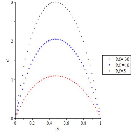
Figure 4 represents the effect of Erying-Powell parameter on the velocity profile. The result shows that decrease in M enhances the velocity profile. This implies that, increase in M decreases the profile.
Figure 1. Effect of the thermal Grashof number on the velocity profile
Figure 2. Effect of mass Grashof number on the velocity profile
Figure 3. Effect of Peclet number on the velocity and temperature profile
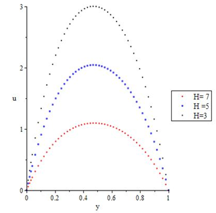
Figure 5 depicts the effect of the Hartmann number on the velocity profile. It is noticed that increase in the value of the Hartmann number decreases the velocity. Thus, this satisfies the fact that increasing Hartmann number decreases the velocity profile due to the production of the resistive force (Lorentz force) which slows down fluid motion within the hydrodynamics boundary layer. Physically, the effect of this resistive force is due to increase in Hartmann number. This established fact is applicable when controlling hot fluid flow during metal processing.
Figure 4. Effect of Eyring-Powell parameter on the velocity profile
Figure 5. Effect of Hartmann number on the velocity profile
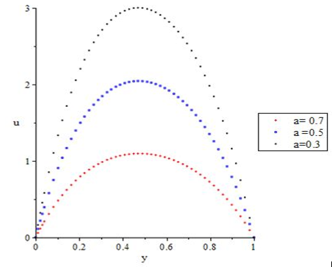
Figure 6. Effect of couple stress parameter on the velocity profile
Figure 6 represents the effect of couple stress parameter on the velocity profile. It is noticed that increase in the couple stress inverse drastically increases the velocity profile. Physically, couple stress inverse on a flow decreases the maximum flow.
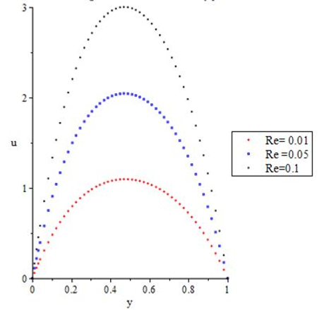
Figure 7. Effect of Reynolds number on the velocity, temperature, and concentration
Figure 7 represents the effect of the inverse Reynolds number on the velocity, temperature and concentration profiles. Obviously, increasing the Reynolds number enhances the velocity profile. This is due to the fact, the viscous force in the non-Newtonian fluid filled up the inertia force. This explains the reason why the velocity is maximum where the inertial force keeps growing and leads to disturbance in the fluid flow, it will result to break down in the laminar flow due to higher Reynolds number. As seen in Figure 7, higher Reynolds number brings increase to the fluid temperature. With increase in the Reynolds number, the concentration profile decreases very close to the wall and continues to behave in an irregular manner as the Reynolds number continues to increase.
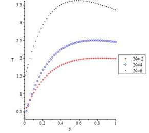
Figure 8. Effect of radiation parameter on the temperature profile
Figure 8 represents the effect of radiation parameter on the temperature profile. Very close to the wall, the temperature profile drastically increases with increase in radiation parameter. Due to the presence of Reynolds number within the fluid the thermal boundary layer enhances with increase in the radiation parameter.
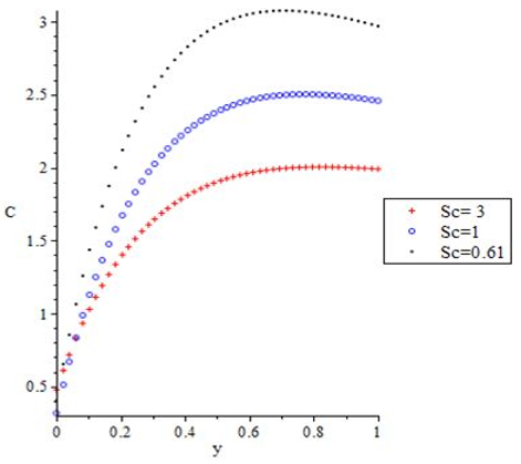
Figure 9. Effect of Schmidt number on the concentration profile
Figure 9 depicts the effect of the Schmidt number on the concentration profile. Schmidt number is the ratio of momentum, to the mass diffusivity. It explains the effectiveness of momentum and mass transport with the hydrodynamics and mass boundary layer. It is observed in Figure 9 that decreasing the values of the Schmidt number increases the concentration profile. Hence, increasing Sc will decrease the mass transport of fluid. It worth mentioning that when Sc=0, it shows the absence of mass transfer.
This investigation considered a non-Newtonian transient incompressible, electrically conducting fluid between two parallel porous plates. The Parallel plates are at distance h apart under the influence of couple stress and externally applied magnetic field. The pressure driven fluid was analysed using Eyring-Powell Non-Newtonian fluid model. The non-linear dimensional partial differential equations, under some assumptions, were transformed into a set of dimensionless equations. The solution to the dimensionless equations were obtained using spectral relaxation techniques (SRM). From this study, it was found that
(i). The magnitude of the velocity increases with increase in the inverse couple stress parameter
(ii). increase in the value of the Hartmann number decreases the velocity
(iii). Flow attains maximum values as thermal Grashof number increases
(iv). increasing the Reynolds number enhances the velocity profile, higher Reynolds number brings increase to the fluid temperature and the concentration profile decreases very close to the wall.
[1] Adesanya, S.O., Falade, J.A., Rach, R. (2015). Effect of couple stresses on hydromagnetic Eyring–Powell fluid flow through a porous channel. Theoretical and Applied Mechanics, 42(2): 135-150. https://doi.org/10.2298/TAM1502135A
[2] Eldabe, N.T.M., Hassan, A.A., Mohamed, B., Mona, A.A. (2003). Effect of couple stresses on the MHD of a non-Newtonian unsteady flow between two parallel porous plates, Z. Naturforsch. 58(a): 204-210. https://doi/10.1515/zna-2003-0405
[3] Srinivasacharya, D., Kaladhar, K. (2012). Free convection flow of couple stress fluid between parallel disks. International Conference on Fluid Dynamics and Thermodynamics Technologies, IPCSIT33, pp. 13-18.
[4] Adesanya, S.O., Ayeni, R.O. (2011). Existence and uniqueness result for couple stress bio-fluid flowmodel via Adomian decomposition method. International Journal of Nonlinear Science, 12(1): 16-24.
[5] Adesanya, S.O., Makinde, O.D. (2012). Heat transfer to magnetohydrodynamic non-Newtonian couplestress pulsatile flow between two parallel porous plates, Z. Naturforsch, 67(a): 647-656.
[6] Zueco, J., B´eg, O.A. (2009). Network numerical simulation applied to pulsatile non-Newtonian flowthrough a channel with couple stress and wall mass flux effects. Int. J. Appl. Math. Mech., 5(2): 1-16.
[7] Tsai, C.C., Hsu, T.W. (2010). Oscillatory Stokes flows in convection and convective flows in porous media. Comput. Fluids, 39: 696-708.
[8] Zakaria, M. (2003). Effects of free convection currents on the oscillatory flow of a viscoelastic fluid with thermal relaxation in the presence of a transverse magnetic field bounded by a vertical plane surface. Appl. Math. Comput. 139: 265-286. https://10.1016/S0096-3003(02)00179-0
[9] Makinde, O.D., Mhone, P.Y. (2005). Effects of radiative heat transfer and magnetohydrodynamics on an oscillatory flow in a channel filled with a porous medium. Rom. J. Phys., 50: 931-938.
[10] Hakeem, A.K.A., Sathiyanathan, K. (2009). Analytical solutions on free convective radiation of an incompressible viscous fluid through a highly porous medium bounded by an infinite vertical plate. Nonlin. Anal., 3: 288-295. https://doi.org/10.1016/j.nahs.2009.01.011
[11] Mahmoud, A., Ali, A. (2007). Unsteady oscillatory flow of an incompressible viscous fluid in a planar channel filled with a porous medium in the presence of a transverse magnetic field. Rom. J. Phys., 52: 85-91.
[12] Idowu, A.S., Falodun, B.O. (2018). Soret-Dufour effects on MHD heat and mass transfer of walter’s-B viscoelastic fluid over a semi-infinite vertical plate: Spectral relaxation analysis. Journal of Taibah University, 13(1): 49-62. https://doi.org/10.1080/16583655.2018.1523527
[13] Alao, F.I., Fagbade, A.I., Falodun, B.O. (2016). Effect of thermal radiation, Soret and Dufor on an unsteady heat and mass transfer flow of a chemically reacting fluid past a semi-infinite vertical plate with viscous dissipation. Journal of the Nigerian Mathematical Society, 35(1): 142-158. https://doi.org/10.1016/j.jnnms.2016.01.002
[14] Oyelami, F.H., Dada, M.S. (2018). Numerical analysis of non-Newtonian fluid in a non-Darcy porous channel, modelling, Measurement and Control, 87(2): 83-91. https://doi.org/10.18280/mmc_b.870204