Identification of Transfer Functions in a Vacuum Brazed Load with ARX Models
Identification de Fonctions de Transfert dans une Charge Brasée sous Vide à Partir de Modèles ARX

Célien Zacharie* | Vincent Schick | Benjamin Remy | Gaëtan Bergin | Thierry Mazet | Renaud Egal
© 2020 IIETA. This article is published by IIETA and is licensed under the CC BY 4.0 license (http://creativecommons.org/licenses/by/4.0/).
OPEN ACCESS
In the context of the study of the thermal behavior of an industrial system composed of an electric vacuum brazing furnace and its load (a plate and brazed heat exchanger), and the control of the associated process, we want to identify and exploit the transfer functions of both elements through ARX models (autoregressive structure). This paper deals with the use of internal transfer functions related to the load and is divided into two parts. First a numerical study will consist of estimating transfer functions on a reference 2D model and quantifying their sensitivity to defaults likely to be encountered on the real process. This method will then be extended to the real system.
RÉSUMÉ :
Dans le cadre de l’étude du comportement thermique d’un système industriel constitué d’un four électrique de brasage sous vide et de sa charge (échangeur thermique à plaques et ondes brasées), et de la maîtrise du procédé associé, on souhaite identifier et exploiter les fonctions de transfert des différents éléments via des modèles paramétriques de type ARX (structure autorégressive). Le présent article concerne l’exploitation de fonctions de transfert internes à la charge (entre sa surface extérieure et son centre géométrique) et se décompose en deux parties. Une étude numérique consistera à estimer des fonctions de transfert sur un modèle 2D de référence et à relever leur sensibilité à des anomalies susceptibles d’être rencontrées sur le procédé réel. Cette méthode sera ensuite étendue au système réel.
heat transfer, system identification, transfer functions, ARX models, vacuum brazing
Mots-clés :
identification de systèmes, fonctions de transfert, modèles autorégressifs, procédé industriel de brasage sous vide
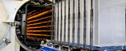
In an industrial context of manufacturing brazed aluminium heat exchangers (BAHX), it is now difficult to distinguish healthy brazed assemblies from defective ones before hydraulic testing; the brazing operation being carried out in an electric vacuum furnace (see Figure 1). This stage of the manufacturing process is based on heating the charge (exchanger) to the melting point of the braze, thus allowing the initial stack to form a solid block. Based on measurements by thermocouples located at certain points in the exchanger, only on the surface and in its core, a series of radiant panels monitored by a control unit heat the load to the soldering temperature while ensuring its thermal homogeneity, the latter being characterized by a temperature difference between the outside and the centre of the charge.
However, the temperature and power data collected do not enable the presence of defaults or brazing anomalies in the exchanger to be detected (due to the emergence of hot spots, for example). A more detailed analysis of the behaviour of the industrial furnace and its load is therefore required.
To solve this problem, we are trying to identify the transfer functions of the vacuum brazing furnace and the load through parametric models of the ARX type (autoregressive structure).
This study will focus on the use of internal transfer functions in the load. First, based on a 2D model of an exchanger passage under FlexPDE® (finite elements), the transfer functions between the surface and the geometric centre estimated from a reference case (without anomaly) will be compared with other cases (with anomaly) likely to be encountered on the real process. These simulations should ensure that the ARX parametric models reconstruct the expected responses at the geometric centre and help identify the sensitivity of these models to simulated defaults in the tests.
Figure 1. Photograph of one of the two on-site furnaces and an exchanger before loading
Based on the previous observations, the rest of the study will be devoted to estimating parametric models on a series of six identical exchangers, based on data provided by the real system. The first one will be chosen as a reference for estimating the transfer functions and the other five will be compared to it. An attempt will then be made to classify the exchangers (their respective brazing cycles) according to the different distributions observed.
Beforehand, we will give more information on how to position the problem in its industrial context and a brief presentation of the ARX autoregressive models.
2.1 The studied system
The overall objective of this research work (in collaboration with Fives Cryo) is to propose a new method for predictive analysis of the behaviour of the electric vacuum brazing furnace according to variable exchanger geometries through the association of transfer functions identified on the real system {furnace + load}.
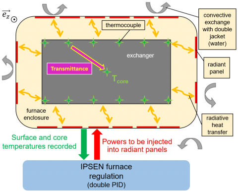
The heat transfer modes involved are radiative (heat transfer between the radiant panels of the furnace and the aluminium exchanger and other additional elements included in the enclosure), conductive (within the load itself), and convective if we consider the furnace enclosure which is a double jacket where water circulates (cold source for regulation). In the enclosure, 88 panels exchange heat by radiation with the load, which is equipped according to its geometry with a few dozen surface thermocouples (exchanger skin) and at least two core thermocouples in the event of a malfunction of one of them. By strategically combining the skin sensors with the panels, i. e. by placing them so that they face each other, the temperature gradient in the load is monitored and controlled during the cycle so that the heating is as homogeneous as possible. With respect to the 6 exchangers studied here, 36 surface sensors were used for each. In the diagram in Figure 2, a heat exchanger in the furnace enclosure, its instrumentation and the associated control strategy are represented in the (x,y) plan. The radiant panels are schematized in red and the temperature sensors in green. An example of transfer function is the transmittance between two points inside the exchanger. As this is a horizontal cross-sectional view, only 16 of the 88 panels have been represented, and the same applies to the 12 of the 36 skin thermocouples.
Figure 2. Horizontal cross-sectional diagram of the system {furnace + load}
The main challenges of this work consist in developing a methodology that will at least make it possible to explain a posteriori the appearance of defaults or anomalies during an elapsed cycle, and ideally to detect them in situ during the process. In this perspective, the approach chosen consists in identifying the transfer functions mentioned via ARX autoregressive parametric models.
2.2 ARX parametric models
A transfer function, which can be considered as the identity card of the studied system, links at least two quantities together. It is possible to estimate this operator which links the response y to its thermal excitation u through a parametric model of type ARX.
Over the last decade, ARX models have seen their use grow in some applied fields, whereas they were previously studied from mathematical and automatic points of views. Many works related to heat transfer problems in building science have used parametric fit methods in order to estimate behavioral laws in an efficient way [1, 2], to build virtual sensors [3-5], or to improve the efficiency of some installations [6, 7]. Furthermore, the use of this tool in the context of process monitoring in the industrial environment is perfectly adapted because parametric models are generally quick to estimate and use [8-10]. Augmented versions of these linear models have been studied in the following research works [11-13].
Autoregressive models can be considered as generalizations of convolution and enthalpy balances, at least in heat transfer domain, as explained by Jauregui et al. [14]. In the same way as for the enthalpy method, the output of an autoregressive model is therefore a variable related to the chosen system, but does not require the explicit writing of the heat balance. Hence this approach is all the more relevant when working on 2D/3D or real systems for which physics is difficult to model finely.
To summarize, in our heat transfer problem, autoregressive models can express more implicit equations from heat balances such as Eq. (1).
$\rho {{c}_{p}}\frac{\partial {{T}_{s}}}{\partial t}=-\sum\limits_{i}{{{G}_{i}}\left( {{T}_{s}}-{{T}_{i}} \right)}+P$ (1)
ρcp denoting the volumic heat capacity of the system, Ts the output temperature of the system, Gi the thermal conductance characterizing the heat transfer between the system and the element i, and P an intern production term of the system.
ARX are exogeneous variable models. They have been extensively studied by Ljung [15] and take the mathematical form of Eq. (2) in the case of a model with a single input u and a single output y:
$\begin{array}{l}
y\left(t_{i}\right)=-\sum_{j=1}^{n_{a}} a_{j} y\left(t_{i}-j \Delta t\right) \\
+\sum_{j=1}^{n_{b}} b_{j} u\left(t_{i}-j \Delta t-n_{k} \Delta t\right)+\varepsilon\left(t_{i}\right)
\end{array}$ (2)
Δt denoting the time step of the model.
The disturbances ε are often modelled as random variables to simulate noise, but in this article, we will keep this term equal to zero since the noise level which has been observed on thermocouple measurements is low. Only inputs u modelling external effects determine the output. The associated inverse problem is to estimate the coefficients aj and bj.
The system identification with a parametric model can be done in two steps:
Zacharie et al. [16] provides more information about the identification of such autoregressive models.
In general, we have sought to identify single input – single output transfer functions Tskin – Tcore (skin-core transmittances), Tskin designating one of the surface thermocouples. In this part, the sampling step of the data sets is 100 s.
The results concerning the identification of the models can be given through comparison plots (Arbitrary Units (A.U.)), residuals (difference between the simulated curve and that given by the ARX model), or the mean square error (eRMS), whose definition is recalled below in Eq. (3). Here, the initial values of the inputs and outputs have been shifted so that they conform to the shape of the model: for u(t)=0, there is y(t)=0 (stationary initial state).
${{e}_{RMS}}=\left\| {{T}_{core}}-y\left( t \right) \right\|=\sqrt{\frac{1}{N}\sum\limits_{j=1}^{N}{{{\left( {{T}_{core}}\left( {{t}_{j}} \right)-y\left( {{t}_{j}} \right) \right)}^{2}}}}$ (3)
where, N is the number of data and y is the output of the model.
Figure 3. Scheme and characteristics of the 2D model
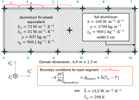
3.1 Presentation of the 2D model and transmittances Tskin– Tcore identification
Thanks to a direct resolution of the 2D model produced with FlexPDE®, temperature profiles can be obtained as a function of time for Tskin (at several locations) and Tcore. The different data sets should then be used to test the sensitivity of the “ideal case” transfer functions to a list of defects and anomalies that may be encountered in reality. This model, whose geometry and different properties are shown in Figure 3, represents a horizontal section of an aluminium exchanger. Boundary conditions include a term simulating the heat flux input of the radiant panels as well as a loss term corresponding to the cooling of the furnace enclosure.
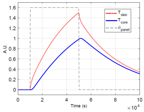
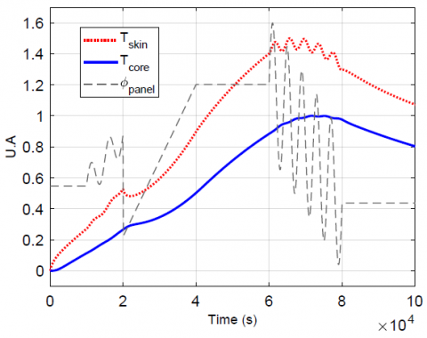
The first issue of this modeling is to verify that the ARX parametric models are adapted to the transfer functions studied. For example, for thermocouple No.2: the calibration and validation signals from the FlexPDE direct reference simulation are those of Figure 4: ϕpanelrepresents the input flux used to obtain Tskin et Tcore for the model calibration (rectangular excitation in Figure 4.a) and its validation (Figure 4.b in which the input flux has a more complex shape).
(a) Calibration dataset
(b) Validation dataset
Figure 4. Input-output datasets for thermocouple No.2
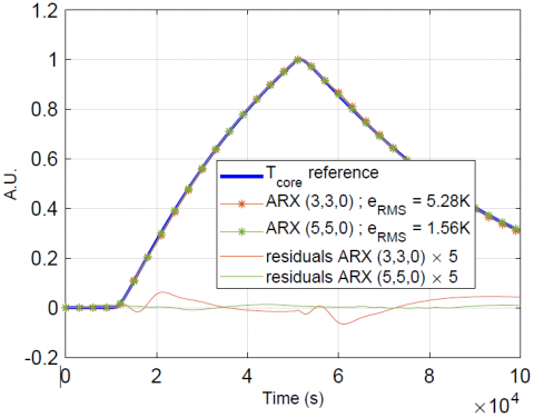
First, we verify whether ARX models can be properly estimated (Figure 5.a), i.e. whether they can correctly reconstruct the reference core response of the direct numerical model. The optimal model is the one that minimizes the RMS criterion on residuals: here the (5,5,0) one.
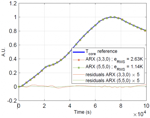
This model is then validated by comparing its output obtained via the complex validation flux with that of the direct simulation (Figure 5.b). Furthermore, this first step made it possible to get ARX models of order 5 that can be tested on the more pathological cases presented afterwards.
(a) Calibration
(b) Validation
Figure 5. 2 ARX models identification (thermocouple No.2)
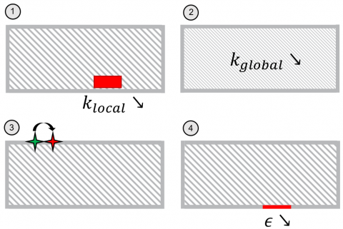
Figure 6. Cavity geometry
3.2 Sensitivity of estimated parametric models to “typical” defaults and anomalies
The four defects (not exhaustive) that have been simulated in FlexPDE are as follows (see Figure 6 for illustration):
1: a decrease of 2 W.m-1.K-1 in conductivity according to x and y directions in a 1m x 0.33m portion near the skin thermocouple n°12 (at the periphery of the exchanger). This choice allows to simulate locally a higher thermal resistance in the modelled exchanger passage;
2: a decrease of 2 W.m-1.K-1 in conductivity in the whole fin-sheet domain according to x and y. This is a generalization of the previous defect to the entire domain;
3: a +8.5 cm position change of thermocouple n°2 in the x direction. During the instrumentation of the exchangers, the location of the thermocouples can vary by a few cm from the set point;
4: a decrease of 2% of wall emissivity around the skin thermocouple n°12 region. In the simulations, this results in a 2% reduction in the thermal power supplied to the concerned area;
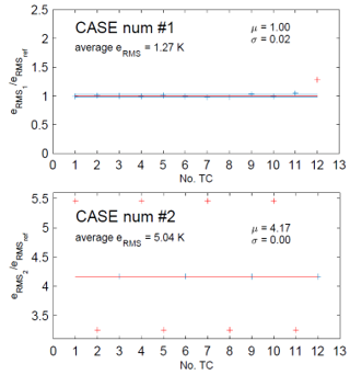
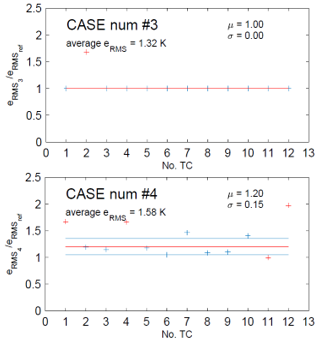
Figure 7. eRMS amplification of the 4 numerical cases
The models estimated in the previous section have been tested by comparing their responses to those of the direct simulations for the 4 cases mentioned above (rectangular excitation for the panels). As there are 12 surface thermocouples in the direct model, 12 reference transfer functions have been estimated. For each anomaly case, the amplification of the model's mean square error amplification has been calculated with respect to the ideal case whose mean eRMS over the 12 thermocouples is 1.17 K. On each graph in Figure 7, each "+" sign corresponds to a thermocouple and its ordinate thus represents the error induced by the simulated defect on its associated Tskin – Tcore transfer function. The mean µ and standard deviations σ of the samples represented by red and blue segments respectively are plotted after a first filtering of the red "+" points placed outside the interval[µ0-σ0 ; µ0+σ0] of the initial sample. For the sake of readability, the y-axis scale is the same for all four graphs.
Comments on the different distributions observed in Figure 7 for each case:
1: the local default has little effect on the thermal paths away from it: only the model linking Tskin n°12 and Tcore does not reconstitute the expected output well, which results in an amplification of the eRMS;
2: a slight modification of the conductivity in the entire domain clearly amplifies the eRMS error to such an extent that the models cannot be considered validated in this case (eRMS 2 = 4.8 K on average.) The severe amplification of the mean square error is therefore global, as might be expected by simulating a default in the whole domain;
3: in case 3, the only failed transfer function is the one whose location of the associated skin thermocouple has been moved, namely No. 2. However, this case cannot be met in reality because the heat exchanger temperature measurements are used in the furnace regulation to develop the power inputs for the panels. The regulation "adapts" to the placement of the thermocouple. To obtain the signature of a real sensor placement defect, the temperature measurement should be "active" on the regulation;
4: in the latter case, the models associated with corner thermocouples No. 1, 4, 7 and 10 are quite sensitive to the 2% decrease in heat flux in the region around thermocouple n°12 because it breaks the symmetry of the problem. ARX models are sensitive since they have been calibrated with symmetrical temperature fields. In addition, the model associated with thermocouple n°12 is logically the main one affected by this simulated decrease in surface emissivity. Overall, the 12 ARX models are sensitive to this anomaly;
Thus, the proposed ARX tool is sensitive to different simulated structural and metrological defaults.
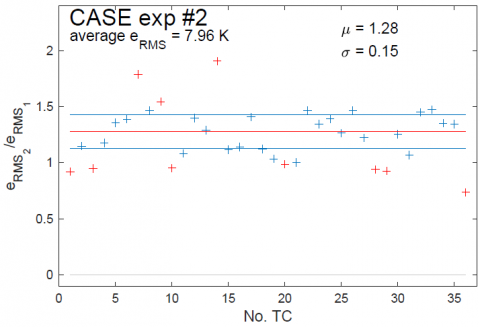
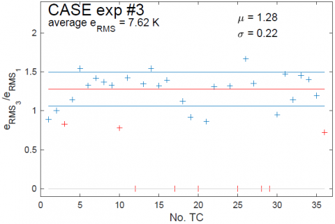
Finally, we would like to compare the brazing cycles of 6 exchangers which share the same geometry. An exchanger is chosen to calibrate the ARX models (5,5,0) and these are tested with the data sets of the other exchangers. Results can then be proposed as root mean square error amplification for the 36 estimated Tskin – Tcore transfer functions. Here, the sampling step of the experimental datasets is 60 s.
It should be noted that the experimental eRMS are not of the same order of magnitude as the numerical ones in the previous section. Indeed, the amplification rates are far from a factor of 5 (average eRMS ref = 1.2 K in section 3 and average eRMS ref = 5.4 K for the real exchanger n°1 considered as reference). In this study, it will therefore not be possible to make a link between the simulated defects and the defects observed in the real cycles.
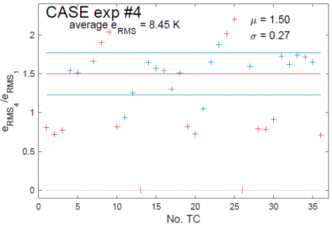
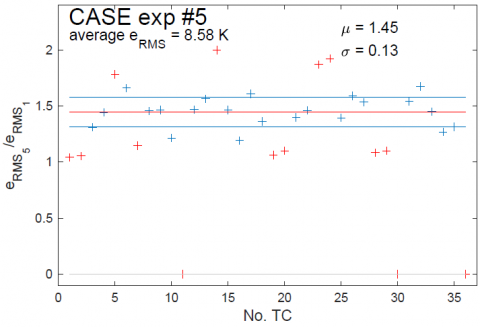
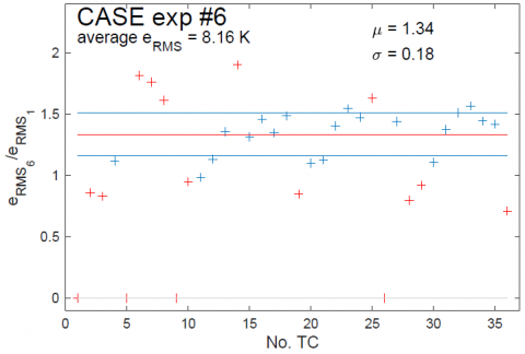
Figure 8. eRMS amplification of the 5 experimental cases
In the graphs in Figure 8, two filters have been applied, the first consisting of excluding malfunctioning thermocouples (the ordinate of the corresponding red "+" being set to zero), the second being the same as in section 3.
Case n°1 has led to the identification of ARX models. Exchangers 2, 3 and 6 are the closest to the reference case (the mean µ of their respective amplification rates are the lowest) despite a larger dispersion in case 3, possibly due to the 6 defective thermocouples that deprived the regulation of thermal information in their associated region. According to the developed observable (eRMS/eRMSref), the cycles of exchangers 4 and 5 are globally further away from the reference exchanger (µ≥1,45). The standard deviation is significantly greater on exchanger n°4, which is eventually the exchanger whose cycle has diverged the most from case n°1. Besides the thermocouples with an amplification rate close to 2 (n°23, 24 and 25) are located in the area assumed to be responsible for the waste of device n°4, with effects on the distribution of the temperature field that generate a dispersion on the response of the models comparable to that of the numerical case n°4.
Thus, through ARX models, the Tskin – Tcore transfer functions identified on a reference case are also sensitive to experimental data and the observable eRMS/eRMSref makes it possible to classify exchangers of the same series according to a reference that is given.
ARX models can represent the heat transfer between the heat exchanger surface and its geometric centre. Based on the numerical model, the sensitivity of this tool to different types of defects has been highlighted. Using experimental Tskin – Tcore transfer functions, the observable eRMS/eRMSref made it possible to compare different brazing cycles with a reference cycle corresponding to a healthy device. In order to deepen the analysis, the model identification methodology will have to take into account the power regulation effects of the panels: the correlations between flux and temperature, although more complex to establish, are likely to provide more information on the occurrence of possible defaults.
This work benefits from the financial support of the company FIVES CRYO as part of a CIFRE collaboration with LEMTA.
[1] Milanović, B., Božić, B., Gospavić., Z., Pejović, M. (2014). Comparison of ARX- and AR-models and of the assumed form of the transfer function when examining settlement of the building. INGEO 6th International Conference on Engineering Surveying, Prague, Czech Republic, pp. 21-26.
[2] Jiménez, M.J., Heras, M.R. (2005). Application of multi-output ARX models for estimation of the U and g values of building components in outdoor testing. Solar Energy, 79(3): 302-310. https://doi.org/10.1016/j.solener.2004.10.008
[3] Mustafaraj, G., Chen, J., Lowry, G. (2010). Development of room temperature and relative humidity linear paramtric models for an open office using BMS data. Energy and Buildings, 42(3): 348-356. https://doi.org/10.1016/j.enbuild.2009.10.001
[4] Wu, S., Sun, J.S. (2012). A physics-based linear parametric model of room temperature in office buildings. Building and Environment, 50: 1-9. https://doi.org/10.1016/j.buildenv.2011.10.005
[5] Ríos-Moreno, G.J., Trejo-Perea, M., Castañeda-Miranda, R., Hernández-Guzmán, V.M., Herrera-Ruiz, G. (2007). Modelling temperature in intelligent buildings by means of autoregressive models. Automation in construction, 16(5): 713-722. https://doi.org/10.1016/j.autcon.2006.11.003
[6] Yu, Y., Woradechjumroen, D., Yu, D. (2014). Virtual surface temperature sensor for multi-zone commercial buildings. Energy Procedia, 61: 21-24. https://doi.org/10.1016/j.egypro.2014.11.896
[7] Yoshida, H., Kumar, S. (2001). Development of ARX model based off-line FDD technique for energy efficient buildings. Renewable Energy, 22(1-3): 53-59. https://doi.org/10.1016/S0960-1481(00)00033-1
[8] Samyudia, Y., Sibarani, H. (2006). Identification of reheat furnace temperature models from closed-loop data – an industrial case study. Asia Pacific Journal of Chemical Engineering, 1(1-2): 70-81. https://doi.org/10.1002/apj.9
[9] Loussouarn, T., Maillet, D., Remy, B., Schick, V., Dan, D. (2018). Indirect measurement of temperature inside a furnace, ARX model identification. Journal of Physics: Conference Series, 1047: 012006.
[10] Sahnoun, B., Remy, B., Schick, V., Lopez, A., Guilbaut, R. (2019). Modélisation et simulation du transfert thermique verre-moule dans un procédé de soufflage verrier. French Heat Transfer Society (SFT) Congress, Nantes, France.
[11] Battaglia, J.L., Le Lay, L., Batsale, J.C., Oustaloup, A., Cois, O. (2000). Utilisation de modèles d’identification non entiers pour la résolution de problèmes inverses en conduction. International Journal of Thermal Sciences, 39(3): 374-389. https://doi.org/10.1016/S1290-0729(00)00220-9
[12] Malti, R., Victor, S., Oustaloup, A. (2008). Advances in system identification using fractional models. Journal of Computational and Nonlinear Dynamics, 3(2): 021401. https://doi.org/10.1115/1.2833910
[13] Johansen, T.A., Foss, A. (1995). Empirical modeling of a heat transfer process using local models and interpolation. Proceedings of 1995 American Control Conference, pp. 3654-3658. https://doi.org/10.1109/ACC.1995.533819
[14] Jauregui, F.U., Remy, B., Degiovanni, A., Verseux, O. (2013). Model identification for temperature extrapolation in aircraft powerplant systems. International Journal of Thermal Sciences, 64: 162-177. https://doi.org/10.1016/j.ijthermalsci.2012.08.019
[15] Ljung, L. (1987). System identification: theory for the user, Models of linear time-invariant systems. Thomas Kailath, Prentice-Hall Information and System Science Seies, 169-115.
[16] Zacharie, C., Schick, V., Remy, B., Bergin, G., Egal, R., Mazet, T. (2018). Transfer functions identification for a brazing furnace and its load. French Heat Transfer Society (SFT) Congress, Pau, France, pp. 536-543.