Kavitha Chellappan* | Denis Ashok Sathiaseelan
© 2020 IIETA. This article is published by IIETA and is licensed under the CC BY 4.0 license (http://creativecommons.org/licenses/by/4.0/).
OPEN ACCESS
The spindle is one of the principle components in machine tools which provide accurate rotational motion to meet appropriate demands. If spindle rotation is not proper, the work piece obtained from that machine will also be inaccurate. In industrial applications, the spindle error motion is analyzed for understanding the performance of machine tools. The evaluation of either of the direction information is utilized for finding the dynamic error motion of the machine tools. The one direction motion information was used for evaluating error motion. In present work, instead of using one direction information, both data are used for analyzing the error motion. This has been done by extracting the spindle edge detail information from the captured sequential image using suitable edge detector. The subpixel level edge is obtained for removal of form error in artifacts. Both direction location of spindle has been utilized by converting the information from cartesian plane to the polar plane. The polar Fourier series is used to find the spindle error and further used to separate the synchronous, asynchronous and centering error motion. Thus finally, for different spindle speed, synchronous error obtained was in range of 4.65um to 7.02 um and asynchronous error as 12.48um to 21.90um.
spindle, polar Fourier, radial error, calibration, image processing, canny edge, subpixel, least square
In the manufacturing world, the spindle is considered as one of the principle components. The spindle provides rotation to the components by making stator as stationary and rotor as rotating. The rotation should be a perfect one to achieve high efficient and accurate work piece during machining. The ideal spindle will have one degree of freedom, whereas in practical case, the machinery spindle contains five degrees of freedom. The five degrees are two in radial direction, one in axial and two in tilt position. The precise rotation of the spindle helps to attain precise product from that particular spindle [1]. If the machine tool spindle rotation is not perfect, the product obtained from that spindle will not be precise enough. In the obtained work piece or product, spindle errors along with form error of the artifact will also accumulate in it. This affects the accuracy and production of products from the machine having such spindles. Many research works had been proposed to measure the spindle errors by using some standards such as ISO 230 part 7, JIS B 6190-7 and ANSI/ASME B89.3.4 [2]. These standards specify the spindle error during motion, degrees of freedom, form error of the target used and also illustrate appropriate ways to segregate the spindle errors.
The spindle runout was measured using dial indicator and in that the spindle errors are embedded with centering error and surface error of the artefact [3]. The dial indicator based spindle error measurement was a contact based measurement and the measurement was carried out on stationary spindle. The rotating spindle error motion and stationary might not produce the same error motion.
Later, the displacement sensors such as inductive and capacitive sensors were used for measuring the spindle runout. In 2010, a regression based method was used to find the spindle radial errors. The input data was acquired from the capacitive sensors placed near the spindle. Since it is a displacement sensor, during rotation, the distance between the spindle and sensor head was acquired and analyzed [4]. In 2015, Zhang et.al, developed a new cylindrical capacitive sensor based approach to find spindle errors in five degrees of freedom. It measures the radial error motion accurately with an eccentricity of 15um. This method also measures the axial and tilt error motion. Even though the sensors provide greater resolution, the usage of displacement sensors were limited by its working distance between the target and the sensor head [5].
In 1990s, the laser based measurement technique was proposed for spindle rotational error motion measurement by passing the laser beam over the surface of the spindle. An appropriate method for measuring radial and angular error motion of different range of speed using laser diode and position sensitive detectors were developed [6]. In 2002, Jywe and Chen presented a simple method by using laser diode and four quadrant sensor. In this developed method, in addition to spindle errors, the spindle speed and indexing can also be noted. The simplicity of this approach is no usage of master target or marks for measuring spindle errors [7].
The method proposed by Liu et. al., proposed a method where the laser diode and batteries are integrated in the rotational fixture which regrets the usage of master target. The motion of laser point was detected using two PSDs on machine tools. The laser beam was split into two separable beams by beam splitter and falls on the PSDs. This information was used to find the spindle radial and tilt errors with some mathematical formulations [8]. This laser based measurement techniques requires a longer period of time in calibration and alignment of path for laser beam and also it requires many components for spindle error measurement setup.
A new algorithm was developed for measuring the spindle error motions. In this, an indexing marker was placed on the spindle for error measurement, which helps to measure the spindle speed in accurate way. The spindle speed was set in the range of 600rpm to 6000 rpm. The developed program uses the sensor information for determining the motion. The developed algorithm followed the international standard for measuring the total error motion, asynchronous and asynchronous spindle errors and also the spindle speed. This method measures the spindle geometric errors and compensated rotation, orientation and straightness error. But here the form error was not taken into account during measuring [9].
Castro (2008) used heterodyne laser interferometer rotation error measurement such radial and axial error motion in a lathe machine. He developed two separate experimental arrangements for measuring radial and axial errors separately. A high precision master sphere has been fixed at the end of wobbling spindle for measuring the spindle error motions. Based on the laser beam reflection from the surface of the sphere, the error measurement is carried out. The dispersion of beam was minimized using a convergent lens in the arrangement which helps to spotlight the laser beam to a dot. The obtained data are plotted in the polar plots and this method provides resolution of 1 nm [10].
In recent years, the machine vision based approach for spindle error measurements are proposed by using some appropriate image processing techniques. The images were captured for a spindle speed of 180-360 rpm. Six such revolution images were used for finding the spindle error motion in machine tools. The acquired error motion depends on the image quality and also image processing algorithms [11].
A new method of finding spindle redial error using machine vision based approach was proposed in 2017 [12]. A standard cylindrical target with 10mm diameter was mounted on the spindle and used as a master target. The sequential frames of the rotating spindle with cylindrical target had been analyzed for finding the spindle radial error in horizontal direction. The captured sequential images were edge detected and subpixel level edge information was obtained using Circular Hough Transform. Further, the data was analyzed using least square fitting for spindle error separation. Here, the error was separated using one co-ordinate axis.
The machine tool spindle rotational accuracy is an important consideration for producing good quality products. The spindle rotational errors were measured by using capacitive, inductive sensors, laser based and vision based systems. In the existing vision based methods, the spindle radial error component was isolated from the centering error and form error of the artifact by using the cartesian plane data. In this work, the spindle runout in one direction that is either horizontal error motion or vertical error motion was considered for analyzing the spindle radial error motion. In the proposed method, both direction information is used for analyzing the error motion by converting the cartesian plane information to polar plane. The form error present in the artifact was removed by circle fitting algorithm. Also in the proposed method, the spindle error motion was analyzed and the centering error, synchronous and asynchronous error motion was separated for different spindle speed.
The proposed machine vision setup consists of a camera, lighting system, frame grabber, computer aided data acquisition system for measuring the spindle radial error motion in a machine tool. The proposed spindle radial error measurement has been carried out in the lathe machine by acquiring the images of the target at different operational speeds. A diameter of 13 mm cylindrical master is fixed on the lathe machine for finding the rotational error of lathe spindle. On the other side, the CMOS camera is fixed on lathe machine tool post for focusing the master cylinder. A positioning stage is used for focusing the camera to the cylindrical master. A standard scale of 100 cm is used for measuring the spacing between the camera and the master target and it was measured to be 40 cm. The machine vision applications require a proper lighting system for image acquisition. The target object has to be illuminated properly before capturing the image. So a ring lighting system with red LED is used to illuminate the cylindrical target.
The spindle radial error motion is measured by using the sequential image frames taken at different spindle speed. The camera used is an AVT Marlin F-131b monochrome camera. This is a monochrome camera with sensor cell size of 6.7 μm both horizontally and vertically. The camera has a maximum image resolution of 1280 horizontal and 1024 vertical pixels and is interfaced to the personal computer using IEEE 1394 frame grabber. The proposed experimental set up is shown in Figure 1.
Figure 1. Experimental setup for spindle radial error measurement using the vision based system
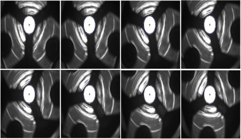
Figure 2. Sequential frames of cylindrical target for spindle speed of 25 rpm
By using the experimental arrangement, the sequential image frames are captured for different spindle speed. Figure 2 shows the sequential frames captured at the spindle speed of 25 rpm.
The spindle radial error motion has to be analyzed by measuring the change in position of the cylindrical target from the sequential images and the error measurement in real world units is to be attained by camera calibration.
2.1 Camera calibration
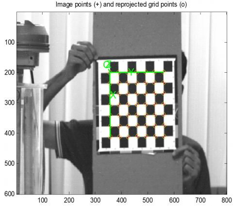
The camera calibration is a fundamental step for machine vision based applications that maps 3-dimensional real world co-ordinates to 2-dimensional image coordinates. There are many methods available to calibrate the camera and for obtaining distortion less view [13]. The commonly used Zhang’s method of 2D calibration approach is used in the proposed method for calibrating the camera [14]. The error occurred due to lens distortion such as radial (pincushion and barrel) and tangential errors have been corrected by using Zhang’s method. The re-projected corners grid points by using the camera calibrations results are shown in Figure 3. In this Figure, the corners are detected automatically using harris corner detection method.
Figure 3. Calibration of checkerboard pattern
2.1.1 Estimation of camera parameters
Once all of the calibration pattern corners are detected by selecting the 4 points on the checkerboard, the intrinsic camera parameters can be obtained and it is shown in the Table 1.
The estimated camera intrinsic parameters give the total radial and tangential distortion of the camera and it is found to be minimum. These values are used for un-distorting the image.
2.1.2 Lens distortion correction
The camera calibration result gives the coefficient of radial (k1,k2,k3) and tangential (p1,p2) lens distortion. Those values are used for correcting radial and tangential distortions in the image. Figure 4 shows the input and the distortion free images. Using the distortion co-efficient, the images are corrected automatically. The distortion vectors show that the camera lens distortion is very low and it could be neglected while using in real time acquisition.
Table 1. Estimated intrinsic parameters of the camera
|
Intrinsic Parameters |
Values |
|
Focal Length |
[7720.796 8038.515] ± [773.234 809.914] |
|
Principal point |
[464.086 316.721] ± 13.913 19.513] |
|
Skew |
[0.00000] ± [0.00000] |
|
Distortion |
[12.24773-10705.72763 -0.02928-0.02428 0.00000] ± [5.56477 7645.66663 0.01658 0.01362 0.00000] |
|
Pixel error |
[0.21403 0.20671] |
Figure 4. Lens distortion correction in the captured image
2.1.3 Scaling factor using estimated camera parameters
Once the distortions of lens are removed, it can be ready for image acquisition. To get the real world units from pixel information, the scaling factor has to be calculated. In this work, the scaling dimensions are obtained using a proper checkerboard pattern with a proper lighting system for acquiring the edge points of square pattern and are shown in Figure 5. From the standard image of checker board pattern of known distance, the scaling values for changing the image pixel data to real world dimension is obtained. Further the number of pixels in horizontal (x) and vertical (y) has also been counted.
$P_{x}=\frac{\text { Dimension of blocks in x direction }}{\text { Number of pixels in x direction }}$ (1)
$P_{y}=\frac{\text { Dimension of blocks in y direction }}{\text { Number of pixels in y direction }}$ (2)
Figure 5 shows the checkerboard of dimension 30mm x 30mm used and the number of pixel counts in horizontal and vertical directions of one black pattern is measured to be 361x360 pixels respectively. Hence the scaling factor to obtain information is real world dimension is found to be 0.083mm/pixel.
Figure 5. Scaling factor from calibrated camera
2.2 Boundary extraction of the cylindrical target
There are many edge detectors available for extracting the boundary of the objects in the digital images [15]. The soft computing based methods are also used for detecting the object boundaries in digital images provided with prior knowledge about the edge [16]. But due to the drawbacks of first and second order derivative based edge detection, the canny edge detector was proposed which uses both concepts for derivative function for smoothing and boundary detection. This detector detects and locates edge points in a proper way with uni-response to an edge point [17]. In canny edge detection, Gaussian filter is first applied for removing high frequency noise content in the image. The upper and lower threshold values are used for locating edge points accurately. Since first and second order edge detector uses one threshold value and sensitive to noise, canny edge detector was used here for detection of edges. The optimized result of edge information can be inferred by first smoothing the image for reducing noise and next by finding the gradient magnitude along horizontal and vertical directions. The magnitude and direction of the gradient G is given by,
$|\nabla I|=G=\sqrt{G x^{2}+G y^{2}}$ (3)
$\theta=\operatorname{atan}\left(G_{x}, G_{y}\right)$ (4)
where, Gx, Gy are the partial derivative of captured cylindrical target image I along horizontal and vertical respectively. The maximum gradient above the threshold are grouped into edge pixels. Figure 4 shows the input image and the result of canny edge detector for the acquired image.
Figure 6(b) gives the edge details that is obtained using gaussian smoothing and derivative functions. The double thresholding in the canny method gives fine edge details compared to other edge detection methods [18]. But however it gives only edge details at pixel level. Hence, in the proposed method, the least square curve fitting algorithm is used for finding the circular target boundary trajectory and for estimating the spindle radial error motion.
Figure 6. Output of canny edge detector for target image
The boundary of the target in the digital image is obtained using canny edge detection operator. Further to view the precise details, subpixel edge information is needed. In the present method, the subpixel edge details are obtained from the image using least square curve fitting method [19]. The least square minimizes the error between the original and predicted data. Further, the residual obtained is also low in least square fitting. The main advantage of this method is simple computing approach. The equation of the circle in linear form can be given as,
$A\left(x^{2}+y^{2}\right)+B x+C y=1$ (5)
To find the circle parameters at subpixel level, it is necessary to find the values of A,B and C. It can be written in matrix form as,
$\left[\begin{array}{c}A \\ B \\ C\end{array}\right]=\left[\begin{array}{lll}\sum_{i}\left(x_{i}^{2}+y_{i}^{2}\right)^{2} & \sum_{i}\left(x_{i}^{2}+y_{i}^{2}\right) x_{i} & \sum_{i}\left(x_{i}^{2}+y_{i}^{2}\right) y_{i} \\ \sum_{i}\left(x_{i}^{2}+y_{i}^{2}\right) x_{i} & \sum_{i}\left(x_{i}^{2}\right) & \sum_{i} x_{i} y_{i} \\ \sum_{i}\left(x_{i}^{2}+y_{i}^{2}\right) y_{i} & \sum_{i} x_{i} y_{i} & \sum_{i}\left(y_{i}^{2}\right)\end{array}\right]^{-1} *\left[\begin{array}{c}\sum_{i}\left(x_{i}^{2}+y_{i}^{2}\right)^{2} \\ \sum_{i} x_{i} \\ \sum_{i} y_{i}\end{array}\right]$ (6)
where, i varies from 1 to total number of edge points. By solving the above equation, the (A,B,C) values are be calculated. Further, by using those values, the circle parameters at subpixel levels by linear methods [20] can be measured as,
$x_{c}=-\frac{B}{2 A}$ (7)
$y_{c}=-\frac{C}{2 A}$ (8)
$r=\frac{\sqrt{4 A+B^{2}+C^{2}}}{2 A}$ (9)
Once the circle center and radius are obtained using least square method, the subpixel edge points has to be calculated and a circle with center (xc,yc) and radius r is fitted over the pixel level data which is obtained from canny edge detector operator.
Figure 7. Edge pixels along X-axis
The target present in the image is circular boundary. The boundary contains, X (Horizontal) and Y (Vertical) pixel information. Thus the fitting along X and Y axis using canny edge detection and least square curve fitting was plotted respectively. Figure 7 and Figure 8 give the least square fitted circle and edge detected circle with center points along X and Y directions.
Figure 8. Edge pixels along Y-axis
The target circle information such as its radius and center location are obtained using least square curve fitting method at subpixel level. The next step is to convert the circle data to polar form. This has to been done to find the spindle radial error along the horizontal and vertical direction during rotation of machine tools. This conversion helps to estimate the two directional spindle error motions in a single attempt. The equation to convert the Cartesian data to polar form is given by,
$m_{i}=\sqrt{x_{p}^{2}+y_{p}^{2}}$ (10)
$\theta_{i}=\tan ^{-1}\left(\frac{y_{p}}{x_{p}}\right)$ (11)
where, (mi,θi) are the magnitude and phase variation between the continuous edge points and (xp,yp) is the subpixel edge information which is obtained from least square curve fitting information. The sequential edge points in polar form can be used further to find the spindle radial error motion data using fourier series. The canonical expression of the fourier series can be written as,
$\left[\begin{array}{c}R_{\theta 1}^{\prime} \\ R_{\theta 2}^{\prime} \\ R_{\theta 3}^{\prime} \\ \cdot \\ \cdot \\ R_{\theta m}^{\prime}\end{array}\right]=\left[\begin{array}{ccccc}1 & \cos \left(1 * \theta_{1}\right) & \sin \left(1 * \theta_{1}\right) & . & \cos \left(k * \theta_{1}\right) & \sin \left(k * \theta_{1}\right) \\ 1 & \cos \left(1 * \theta_{2}\right) & \sin \left(1 * \theta_{2}\right) & . & \cos \left(k * \theta_{2}\right) & \sin \left(k * \theta_{2}\right) \\ 1 & \cos \left(1 * \theta_{3}\right) & \sin \left(1 * \theta_{3}\right) & . & \cos \left(k * \theta_{3}\right) & \sin \left(k * \theta_{3}\right) \\ \cdot & \cdot & \cdot & \cdot & \cdot & \cdot \\\cdot & \cdot & \cdot & \cdot & \cdot & \cdot \\ \cdot & \cos \left(1 * \theta_{m}\right) & \sin \left(1 * \theta_{m}\right) & \cdot & \cos \left(k * \theta_{m}\right) & \sin \left(k * \theta_{m}\right)\end{array}\right]\left[\begin{array}{c}r_{1} \\ a_{1} \\ b_{1} \\ \cdot \\ \cdot\\ a_{k}\ \\ b_{k}\end{array}\right]$ (12)
where, k is harmonic number which varies from 1 to m. r is obtained from mean of radius which is calculated from the Eq. (12). The component (a,b) is the amplitude of cosine and sine terms for Fourier harmonics which is obtained using the below equations,
$a_{k}=\frac{2}{n} \sum_{i=1}^{n} r_{i} \cos \left(i . \theta_{i}\right)$ (13)
$b_{k}=\frac{2}{n} \sum_{i=1}^{n} r_{i} \sin \left(i . \theta_{i}\right)$ (14)
where, n, is the entire number of points in polar curve.
The Eq. R(θ) gives the total error motion of spindle with the inclusion of centering error, radial synchronous and asynchronous error motions.
The total error motion of the machine tool lathe spindle is obtained for different spindle speed of 25 rpm, 50 rpm, 75 rpm and 100 rpm.
Figure 9 shows the total spindle error obtained for different spindle speed. The next step is to segregate the spindle radial error motion from the entire error motion. The total error motion is comprised of synchronous error, asynchronous error and centering error motion. The deviation of the target circle from the base circle is termed as centering error. The synchronous error which is repeatable affects the roundness of the product obtained from that machine tool spindle. The asynchronous error motion is aperiodic and non-repeatable that affects the surface finish of the product. Thus to measure the spindle radial errors, these total error motion has to be separated [21].
5.1 Separation of Spindle radial error components
The polar Fourier series accumulates the total spindle error motion components. It has to be separated for getting spindle radial error motion components. The plot is plotted by finding the number of harmonic components. The number of harmonics relies on the spindle rotational speed and the total number of sequential frames captured for each and every rotation of different spindle speed. Among the total harmonics, the first harmonic component gives the centering error of the spindle which is nothing but the eccentricity [21]. The remaining harmonics give the spindle synchronous error and the residuals obtained from the obtained and the determined gives the non-repeatable error component that is asynchronous error motion. The Eq. (15) gives the centering error which is the first harmonic component.
Centering error $=a_{1} * \cos (1 * \theta)+b_{1} * \sin (1 * \theta)$ (15)
The remaining harmonics gives the synchronous error motion of the spindle and is measured using the below equation,
Synchronous error $=\sum_{j=2}^{k} a_{j} \cos (j . \theta)+b_{j} \sin (j . \theta)$ (16)
Further, the asynchronous spindle error motion which is non-repeatable is measured by subtracting the measured data from the original data.
Asynchronous error $=R_{\theta-} R_{\theta}^{\prime}$ (17)
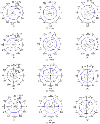
Figure 9. Spindle error motion for the operational speed of (a) 25 rpm, (b) 50 rpm, (c) 75 rpm and (d) 100 rpm
Figure 10. (i) Centering error, (ii) Asynchronous error and (iii) Synchronous error motion for spindle speed of (a) 25 rpm, (b) 50 rpm, (c) 75 rpm and (d) 100 rpm
Table 2. Spindle error motion for different spindle speed
|
Spindle Speed (rpm) |
Synchronous error(µm) |
Asynchronous error (µm) |
||||
|
Data set 1 |
Data set 2 |
Data set 3 |
Data set 1 |
Data set 2 |
Data set 3 |
|
|
25 |
6.509 |
4.580 |
7.826 |
13.21 |
10.76 |
13.47 |
|
50 |
7.078 |
6.811 |
7.166 |
17.39 |
27.43 |
12.92 |
|
75 |
5.732 |
6.016 |
5.223 |
25.96 |
16.68 |
22.24 |
|
100 |
4.548 |
4.356 |
5.042 |
19.89 |
22.20 |
23.60 |
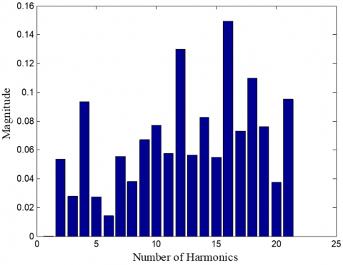
The shift from the base circle in Figure 8.(i) denotes the presence of centering error and it was removed from the spindle radial error components. The harmonic components define the number of lobes in the circular shape. If the harmonic is one, the shape of an object is circular. The harmonic measured from the sequential image indicates the spindle error motion of the machine tool. The magnitude of the harmonics depends on the (a,b) co-efficient values which spots the non-repeatable components of the machine tool. Figure 10 shows the separated error motion for different spindle speeds. And the harmonic components for the spindle speed of 25 rpm are depicted in Figure 11.
The separated spindle radial error components for four different spindle speed have been measured for continuous rotation of the cylindrical target. The Table 2 gives the synchronous and asynchronous spindle radial error motion for four different spindle speeds. For each speed, three sets were taken for analyzing the repeatability of the proposed method.
From the table, it is clear that, with increase in the spindle speed, the periodic error motion is decreasing. This is due to the inner alignment of bearings to that of axis of rotation of the spindle. At the same time, the non-periodic error motion which is asynchronous is increasing with respect to the spindle speed. Thus, if the data is processed in cartesian plane directly, the radial error obtained might contain the combination of error along horizontal and vertical directions. But in this work, the cartesian information is converted to polar information and the spindle errors along horizontal and vertical directions has been measured separately.
Figure 11. Harmonic components for the spindle speed of 25 rpm
In this paper, the spindle radial error motion was measured by converting the data to polar form. This conversion helps to analyze the radial error motion either in horizontal and vertical directions. Further, the spindle errors are separated from the total error motion by using polar fourier series. The centering error was removed by using the first harmonic data. The remaining harmonic component gives the synchronous error and it is varying in the range of 4.3 to 7.8 microns. The residual which is obtained from the polar converted magnitude and the determined values from the polar fourier series gives the asynchronous spindle radial error motion. This error value varies randomly for different spindle speed due to non-periodic nature and it ranges from 10.7 to 27.4 microns. Thus the proposed method helps to analyze the horizontal and vertical spindle radial error motion in single step using the sequential images captured for different spindle operational speed and the extracted data from the sequential images are analyzed using polar fourier series.
[1] Marsh, E.R. (2010). Precision spindle metrology. DEStech Publications, Inc., Lancaster, PA, 161 pages. https://doi.org/10.1115/1.2944275
[2] American National Standards Institute. (1986). Axes of Rotation: Methods for Specifying and Testing. American Society of Mechanical Engineers.
[3] Scheslinger, G. (1978). Testing Machine Tools: For the Use of Machine Tool Makers, Users, Inspectors, and Plant Engineers. Pergamon Press; 8th edition, 109 pages.
[4] Ashok, S.D., Samuel, G.L. (2010). Regression method for identifying spindle radial errors of a miniaturized machine tool. Journal of Studies on Manufacturing, 1(1): 26-33.
[5] Zhang, M., Wang, W., Xiang, K., Lu, K., Fan, Z. (2015). Simulation on measurement of five-DOF motion errors of high precision spindle with cylindrical capacitive sensor. Proceedings Volume 9446, Ninth International Symposium on Precision Engineering Measurement and Instrumentation, 94461L. https://doi.org/10.1117/12.2180823
[6] Park, Y.C., Kim, S.W. (1994). Optical measurement of spindle radial motion by moiré technique of concentric-circle gratings. International Journal of Machine Tools and Manufacture, 34(7): 1019-1030. https://doi.org/10.1016/0890-6955(94)90032-9
[7] Jywe, W.Y., Chen, C.J. (2005). The development of a high-speed spindle measurement system using a laser diode and a quadrants sensor. International Journal of Machine Tools and Manufacture, 45(10): 1162-1170. https://doi.org/10.1016/j.ijmachtools.2004.12.002
[8] Liu, C.H., Jywe, W.Y., Lee, H.W. (2004). Development of a simple test device for spindle error measurement using a position sensitive detector. Measurement science and Technology, 15(9): 1733. https://doi.org/10.1088/0957-0233/15/9/009
[9] Jemielniak, K., Chrzanowski, J. (2015). Spindle error movements measurement algorithm and a new method of results analysis. Journal of Machine Engineering, 15(1): 25-35.
[10] Castro, H.F.F.D. (2008). A method for evaluating spindle rotation errors of machine tools using a laser interferometer. Measurement, 41(5): 526-537. https://doi.org/10.1016/j.measurement.2007.06.002
[11] Deakyne, T.R., Marsh, E.R., Lehman, J., Bartlett, B., Solutions, C. (2008). Machine vision with spindle metrology using a CCD camera. IMAGING, 180, 360RPMs.
[12] Kavitha, C., Ashok, S.D. (2017). A new approach to spindle radial error evaluation using a machine vision system. Metrology and Measurement Systems, 24(1): 201-219. https://doi.org/10.1515/mms-2017-0018
[13] Remondino, F., Fraser, C. (2006). Digital camera calibration methods: Considerations and comparisons. International Archives of Photogrammetry and Remote Sensing, 36(5): 266-272.
[14] Zhang, Z. (2000). A flexible new technique for camera calibration. IEEE Transactions on Pattern Analysis and Machine Intelligence, 22(11): 1330-1334. https://doi.org/10.1109/34.888718
[15] Shrivakshan, G.T., Chandrasekar, C. (2012). A comparison of various edge detection techniques used in image processing. International Journal of Computer Science Issues (IJCSI), 9(5): 269.
[16] Senthilkumaran, N., Rajesh, R. (2009, October). Image segmentation-a survey of soft computing approaches. In 2009 International Conference on Advances in Recent Technologies in Communication and Computing, Kottayam, Kerala, India, pp. 844-846. https://doi.org/10.1109/ARTCom.2009.219
[17] Ding, L., Goshtasby, A. (2001). On the canny edge detector. Pattern Recognition, 34(3): 721-725. https://doi.org/10.1016/S0031-3203(00)00023-6
[18] Rong, W., Li, Z., Zhang, W., Sun, L. (2014). An improved CANNY edge detection algorithm. In 2014 IEEE International Conference on Mechatronics and Automation, Qingdao, China, pp. 577-582. https://doi.org/10.1109/WCSE.2009.718
[19] Xu, G.S. (2009). Sub-pixel edge detection based on curve fitting. In 2009 Second International Conference on Information and Computing Science, Manchester, UK, pp. 373-375. https://doi.org/10.1109/ICIC.2009.205
[20] Solow, D. (2007). Linear and nonlinear programming. Wiley Encyclopedia of Computer Science and Engineering. https://doi.org/10.1007/978-3-319-18842-3
[21] Ashok, S.D., Samuel, G.L. (2012). Modeling, measurement, and evaluation of spindle radial errors in a miniaturized machine tool. The International Journal of Advanced Manufacturing Technology, 59(5-8): 445-461. https://doi.org/10.1007/s00170-011-3519-8