Yinggang Shi | Haijun Wang | Tian Yang | Li Liu | Yongjie Cui*
© 2020 IIETA. This article is published by IIETA and is licensed under the CC BY 4.0 license (http://creativecommons.org/licenses/by/4.0/).
OPEN ACCESS
During greenhouse operations, robots need a specific working path to perform high-precision cruises, and thus, we designed a navigation positioning system based on an odometer/lidar. The navigation positioning system consists of a supervision terminal and a mobile robot. The supervision terminal releases map composition and cruise tasks, and the mobile robot composes a two-dimensional environment map, plans the cruise path and engages in navigation positioning; together, the two perform remote data exchanges through a wireless network. The robot could collect encoder data and obtain mileage information through track deduction, and combined with lidar data and the Gmapping algorithm, a two-dimensional environmental map was established. This system employs an A* algorithm to plan the cruise path and uses AMCL to estimate the position and pose of the robot. Based on the application of an expandable A* algorithm in the navigation toolkit of ROS, a specific working path cruise could be performed by setting goal points. The test results show that the navigation positioning system could perform a specific working path cruise; the average deviation in its straight line walk is 3.34 cm. The average deviation in the specific working path cruise is 2.73 cm, and the system has relatively higher navigation positioning precision because it could finish the specific path cruise and could better satisfy the greenhouse navigation positioning requirements than previous options.
greenhouse robot, simultaneous localization and mapping (SLAM), odometer, lidar, working path cruising
The greenhouse robot is an important piece of technical equipment in the modern greenhouse [1, 2], and automatic navigation technology is a key greenhouse robot technology that could reduce the repetitive operation of robots, reduce costs, and lessen the labor intensity and workload of farmers [3]. Therefore, many experts and scholars have performed relevant studies on navigation positioning technology in greenhouse robots [4, 5]. The navigation positioning technology presently used by greenhouse robots primarily includes interior conventional navigation positioning technology [6-9] and simultaneous localization and mapping (SLAM) [10, 11]. The basic principles of the conventional navigation positioning technology of interior robots is that a robot that moves within a given environment employs Wi-Fi [6, 7], inertial navigation [8] and sensing systems such as visual navigation [9] to cover the room, obtain information on the operational environment and set the navigation parameters of the robot through calculation and motion planning, and then track the preset navigation path of the robot and perform real-time corrections. For example, for the interior positioning system of a robot based on Wi-Fi, it is necessary for the robot to obtain more than 3 wireless sensing signals periodically, and according to the strength of the signal, to analyze its own position after the calculation, which involves a relatively large calculation and test workload [12]. For the interior positioning system of a robot based on inertial navigation, an accelerometer and spiral instrument are applied to calculate the voyage, which could predict the current position and the position of the next step of a mutual robot, and with the continued voyage, the positioning error would accumulate and the positioning precision would decline [13]; for an interior positioning system based on vision, images of the surroundings are collected through cameras, and the information would be fed back to the learning subsystem composed of a neural network and statistical method, the imaged information and the real position of the robot would be connected through the learning subsystem, and thus the autonomous navigation positioning would be completed. If the information is collected by a camera only, the power of the distance-measuring sensor of the active light source is relatively low, which would easily be disturbed by environmental light, and the distance measuring sensor of a non-active light source would barely work under weak light [14]. Simultaneous localization and mapping (SLAM) [10, 11] includes the construction of a two-dimensional environment map, path planning and positioning. While moving in an unknown environment, the robot would estimate its position and pose according to sensor data such as the depth camera, radar, ultrasonic component and encoder, would draw the environment map, and then further perform navigation and positioning, but this technology is rarely applied to greenhouse operations [15]. SLAM technology could effectively help the orchard and robot in greenhouse operation to stop relying on navigation signals and inertial navigation, thus engaging in autonomous operations [16]. Simultaneously, the environment map could be applied to conduct environmental perception and for the precision navigation and positioning of the robot, thus supporting autonomous operation over the entire greenhouse environment.
Greenhouse plants are commonly characterized by “row planting”, and the greenhouse robot needs to complete a traversal cruise of the whole greenhouse by moving through the aisles row by row. For example, during the cruise to pick greenhouse tomatoes shown in Figure 1, the operational goal points of the robot are evenly planned along each aisle, and the robot would reach the goal points one by one. The actuator would finish the operation within the working range and continue to seek and reach the next goal point, and ultimately the robot would complete its cruise of a specific working path. During the autonomous working process, the operational precision of a greenhouse robot is closely connected to its positioning precision, and the positioning precision of walking along the aisle is key to a specific path cruise.
Figure 1. Navigation and positioning of a greenhouse tomato operation (1. Stops during robot operation; 2. cruise path of robot; 3. Tomato planting ridge; 4. aisle between ridges)
To improve the walking precision of a greenhouse robot during its cruise on planned paths, in this article, the encoder has been adapted to collect chassis motion information from a collective wheeled robot, and the mileage information could be obtained through track derivation and then combined with lidar data and the Gmapping algorithm. A two-dimensional environment map would be established in which the odometer is composed of an encoder and the chassis controller of the robot. The AMCL algorithm is applied to position the robot in the map, the A* algorithm is applied to support the overall path plan of the robot, and the DWA algorithm is applied to perform dynamic obstacle avoidance during practical operation. The results show that the precision of that navigation positioning system could satisfy the requirements of a greenhouse operation.
2.1 Greenhouse robot architecture
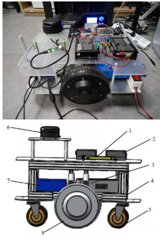
To construct the greenhouse robot as shown in Figure 2, the chassis of the robot is based on a simple McPherson suspension structure, and an aluminum profile (SD-8-3030, SDAL Co., Ltd, Shanghai, China) is used. The in-wheel motors on the left and right (42BL80S09-230TR9, Time Chaoqun Technology Co., Ltd, Beijing, China) are fixed on the frame through a spring shock absorber (31 cm, Car Sales Shop Co., Ltd, Fuan, China) and the two supporting universal wheels on the front and back (2 inch, HUIYIJIAOLUN Co., Ltd, Dongguan, China) play a supporting role, and thus the system has better bearing and surface passing abilities.
Figure 2. Global mechanical structure design of the greenhouse robot chassis (1. Chassis controller of the robot 2. Motor driver 3. Adjustable spring suspension 4. Industrial computer 5. Universal wheel 6. Lidar 7. Power 8. In-wheel motor)
Figure 3. Chassis control system architecture of greenhouse robot
The frame of the chassis control system of the greenhouse robot is shown in Figure 3, and it includes a PC supervision terminal (T3900D, Lenovo Co., Ltd, Beijing, China), a router (F9, Tenda Co., Ltd, Shenzhen, China), an industrial computer (HT780-i5, ZHANMEI Co., Ltd, Shenzhen, China), lidar (RPLIDAR A2, SLAMTEC Co., Ltd, Shanghai, China), a chassis controller of the robot (STM32F103 VET6, Guangzhou Xingyi Electronic Technology Co., Ltd, Guangzhou, China), a motor driver (LSDB4850-CAFR-ALL2, AMPS Co., Ltd, Shenzhen, China), an in-wheel motor and other parts. The industrial computer is the primary controller of the robot, and it has an Ubuntu 16.04 operating system and an ROS system (ROS Lunar Loggerhead). The PC supervision terminal can correspond with the industrial computer through the Wi-Fi provided by the router and obtain motion information about the robot. Then, the PC supervision terminal releases the order of composition, the chassis controller collects signals from the encoder, and the mileage information and motion pose of the robot are obtained through track derivation, which would be sent to the industrial computer through the serial port. The industrial computer integrates the mileage information and laser observation data and then constructs the two-dimensional map of the working environment. After receiving the cruise order from the PC supervision terminal, the industrial computer engages in path planning and send the robot operation order to the chassis motion controller, which then sends the motion control information to the driver of the in-wheel motor. This information drives the rotation of the left and right in-wheel motors on the robot chassis, and thus, the navigational positioning and path cruise of the robot is performed.
2.2 Kinematics analysis of greenhouse robot
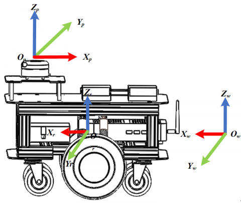
The kinematic model of the greenhouse robot is shown in Figure 4. The world coordinate system Ow-XwYwZw is established at the motion starting point, the robot coordinate system Or-XrYrZr is established at the geometric center of the chassis, and the radar coordinate system Op-XpYpZp is established at the geometric center of the lidar.
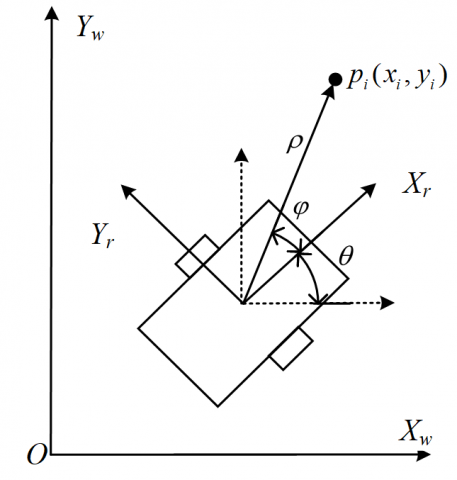
Greenhouse roads are relatively flat, and on the three coordinate systems, the fluctuation values ∆Z of the robot in the direction of the z axis are all relatively small. Therefore, this study only accounts for the motion change in the direction of the X and Y axes, that is, the value ranges of the robot’s greenhouse positioning and navigation are all within the XOY surface of the three coordinate systems. Thus, Xr=[xr(k),yr(k),θr(k)] is applied to represent the pose of the robot, as shown in Figure 5, (xr(k),yr(k)) represents the coordinates of the robot in the world coordinate system Ow-XwYwZw, θr(k) represents the angle between the Xraxis of robot and world coordinate system Xw, the clockwise direction is set as positive, and the anticlockwise direction is set as negative.
Figure 4. Coordinate systems of the robot
Figure 5. Pose model of the robot
The robot has two-wheel drive, the track between the left and right wheel is a, the chassis controller of the robot would read the output pulse of the encoder on the in-wheel motor, and the linear speed of the left wheel Vl and Vr of the right wheel could be obtained after calculation. The two-wheel differential motion model of the robot is shown in Figure 6, and thus the linear and angular speeds of the chassis center of the robot are as follows:
$V_{m}=\frac{V_{r}+V_{l}}{2}$ (1)
$W=\frac{V_{r}-V_{l}}{\mathrm{a}}$ (2)
Combined with the linear and angular speeds of the robot, the odometer model shown in Figure 7 would be established, in accordance with the pose of the two-wheel differential robot after ∆t could be obtained. When setting the linear speed as Vm and the angular speed as W, the distance the robot covers during this time interval is ∆Dk=Vm∆t, and then the angular change with respect to the original point is ∆θk=W∆t. At that very moment, the robot pose is Xr=[xr(k),yr(k),θr(k)], and after ∆t, the robot pose is Xr=[xr(k+1),yr(k+1),θr(k+1)].
Figure 6. Two-wheel differential motion model of the robot
Figure 7. Odometer model
Figure 8. Laser observation model of the robot
Robot motion within a short time period could be regarded as an arc motion, the radius of arc is $r_{k}=\frac{\Delta D_{k}}{\Delta \theta_{k}}$, $\Delta \theta_{k} \neq 0$, and then the robot pose could be obtained through the following odometer model:
$\left[\begin{array}{c}x_{r}(k+1) \\ y_{r}(k+1) \\ \theta_{r}(k+1)\end{array}\right]=\left[\begin{array}{c}x_{r}(k)+r_{k}\left(\sin \left(\theta_{r}(k)+\Delta \theta_{k}\right)-\sin \theta_{r}(k)\right) \\ y_{r}(k)+r_{k}\left(\cos \left(\theta_{r}(k)+\Delta \theta_{k}\right)-\cos \theta_{r}(k)\right) \\ \theta_{r}(k)+\Delta \theta_{k}\end{array}\right]$ (3)
When the robot moves in a straight line within a short time period, $\Delta \theta_{k}=0$, and the robot pose at this time is
$\left[\begin{array}{c}x_{r}(k+1) \\ y_{r}(k+1) \\ \theta_{r}(k+1)\end{array}\right]=\left[\begin{array}{c}x_{r}(k)+\Delta D_{k} \cos \theta_{r}(k) \\ y_{r}(k)+\Delta D_{k} \sin \theta_{r}(k) \\ \theta_{r}(k)\end{array}\right]$ (4)
Error accumulates while estimating the pose of the greenhouse robot with the odometer model only, which would not satisfy the precision requirements of robot navigation and positioning [17, 18]. Therefore, this article adopts lidar to correct the accumulated error of the odometer and perceive the robot environment. The laser observation model of the robot is shown in Figure 8.
The coordinate of the feature point in the lidar detection environment is pi(xi, yi), we set the distance between the feature point of the lidar detection environment and the lidar as ρk,i and the positive angle between the feature point of the lidar detection environment and the lidar is φk,i. Combined with the odometer model, by calculation, the current pose Xr=[xr(k),yr(k),θr(k)] could be obtained, and thus, the robot pose in polar form is
$\left[\begin{array}{c}\rho_{k, i} \\ \varphi_{k, i}\end{array}\right]=\left[\begin{array}{c}\sqrt{\left(x_{r}(k)-x_{i}\right)^{2}+\left(y_{r}(k)-y_{i}\right)^{2}} \\ \arctan \frac{y_{r}(k)-y_{i}}{x_{r}(k)-x_{i}}-\theta_{r}(k)\end{array}\right]$ (5)
2.3 Environment map composition and AMCL positioning
To complete a specific robot path cruise in a greenhouse, it is first necessary to construct a high-precision map under that condition. The ability to perform autonomous positioning in the environment is necessary. Therefore, in this study, the high-precision, two-dimensional grid environment map of the robot in an unknown environment is established based on the Gmapping algorithm of the particle filtering principle [19, 20], and the AMCL algorithm is applied to support the high-precision positioning of the robot. The principles underlying the Gmapping algorithm are as follows:
(1) The initialization stage: the robot begins to move, and certain amounts of particles are set within the unknown map (each particle is a sample, including the map constructed on the basis of the lidar scanning data towards the path and information of the pose), which are scattered evenly over the whole map, and the robot calculates its current pose based on current lidar data and saves it in the particle.
(2) Transfer stage: the robot estimates the state of each particle according to the state transition equation, and the chassis controller of the robot would collect encoder data; then, combined with the odometer model, the pose of the robot during the next moment is estimated, and the particle corresponding to each predicted pose is produced.
(3) Decision stage: the robot continues to advance, the scanning lidar data are compared with the predicted particle, and the weight of the predicted particle close to real conditions is increased. The weight of the predicted particle with a large difference from the real value would be decreased.
(4) Resampling stage: particles with large weights would remain, and those with small weights would be eliminated, leaving particles close to the real pose, and they would continue to complement new particles, to keep the total number the same.
(5) Filtering stage: the system continues to perform a loop iteration of the resampled particles, and eventually, most particles gather in the area most close to the real value to obtain the accurate position of the robot and perform positioning in an unknown environment.
(6) Map generation stage: each particle carries one path map, and thus the two-dimensional grid map under that environment is obtained by combining the particles that are going through the filtering stage.
The robot uses the Gmapping algorithm to construct an environment map of the current position, and it is necessary to invoke real-time scanning lidar and odometer data and then combine them with the mathematic model to estimate its pose so the two-dimensional grid map information could be output. In the ROS system, the message flow is shown in Figure 9. There is an input of the coordinate conversion relation of the robot and radar scanning data into the Gmapping node, and the node would output a two-dimensional map, the dispersion degree of the pose estimation and the corrected error. The launch document of the starting node is then edited according to the following flow chart.
To determine the position of the robot in the map precisely within a specific path cruise, the AMCL algorithm is used in this article for the autonomous positioning of the robot.
Figure 9. Message flow diagram
The AMCL is a plane orientation algorithm based on a probability model, and it is obtained through an improvement in Monte Carlo Localization (MCL). The positioning principle of AMCL is that on the basis of a given map, and combined with laser data and odometer information, a limited particle number is used to represent the possible distribution of robot poses in the environment, and each particle represents one possible robot state. While receiving new sensor data, each particle would estimate its precision by checking its possibility of receiving a sensor number under the current pose. During the action that follows, that algorithm would resample particles to obtain more precise particles. A loop iteration of robot motion for obtaining sensor data and resampling procedures would be continued, and when the positioning succeeds, all the particle swarms would gather near the real pose of the robot. Compared with the MCL algorithm, the ACML integrates odometer information, solves the problem that the overall robot positioning would fail in an unknown environment, and improves the stability and accuracy of robot positioning on the map. The AMCL employs the KLD sampling algorithm to adjust the number of particles dynamically, which to some extent solves the serious increase in the calculations caused by the increased particle number. The essence of the KLD sampling algorithm is to distribute various KL distances by observing two possibilities. The approximation error between KL distance distribution possibility p and possibility distribution q is
$K(p, q)=\sum_{x} p(x) \log \frac{p(x)}{q(x)}$ (6)
The KL distance is a nonnegative number, and when the possibility distribution of p and q are consistent, K(p,q) is zero. Suppose that k subspace possibilities are in discrete distribution, use vector X={X1,X2,…,Xk} to represent the number of sampled particles in each subspace and vector P={p1, p2,…, pk} to represent the real possibility of each subspace, and then the possibility density of its maximum likelihood estimation could be represented as $\hat{P}=X / n$. When the n particle number meets certain conditions, the KL distance K(p,q) between the estimated possibility distribution and real possibility distribution could be set at smaller than the upper limit value ε, which also guarantees that the error between the estimated possibility distribution and real possibility distribution is the minimum; according to the Wilson-Hilferty transition, the equation for dynamic particle number n in the KLD that makes the approximation error the minimum is
$n=\frac{k-1}{2 \varepsilon}\left\{1-\frac{2}{9(k-1)}+\sqrt{\frac{2}{9(k-1)}} z_{1-\delta}\right\}^{3}$ (7)
The z1-δ in the equation is a standard normal distribution with an upper quantile of 1-δ, and it could be understood that particle number n is inversely proportional to upper limit vale ε and proportional to subspace number k. In the KLD algorithm, new particles would continue to be produced until they are larger than particle number n or the user-defined upper limit. This dynamic selection method reduces the particle number and the calculation of the algorithm, and at the same time, the possibility distribution could be relatively accurate.
Figure 10. Communication architecture of the AMCL positioning node
The communication architecture of the AMCL positioning node is shown in Figure 10. The AMCL positioning node would be operated in the ROS, and it would autonomously subscribe/map the topic, /scan lidar would scan the data and /odom odometer information. The MCL based on the possibility model would initialize the particle swarm, estimate the robot motion of robot according to the motion model, and modify the importance weight through a measuring update, so as to strengthen the weight of the particles for the correct pose and restrain the weights of particles in the wrong pose, so as to estimate the pose of the robot within the overall situation. Calculating the number of necessary particles through KLD adaptive sampling could increase the utilization ratio of the particles, and reduce the particle redundancy, and finally, the AMCL positioning node would release the positioning information for the /amcl_pose robot.
2.4 Global path planning and dynamic obstacle avoidance
While performing a high-precision specific path cruise, the robot not only needs to complete the map composition and positioning but also has to be able to engage in autonomous navigation and path planning. This autonomous navigation and path planning primarily includes global path planning and dynamic obstacle avoidance. Therefore, this article adopts the global path planning algorithm based on the A* algorithm and dynamic obstacle avoidance based on DWA (Dynamic Window Approach, DWA). The optimal path the robot takes to reach the appointed goal point could be calculated through global path planning, and the dynamic obstacle avoidance algorithm could engage in the dynamic adjustment of the global path, and perform an obstacle avoidance function during the process of reaching the appointed goal point.
The principle of the A* algorithm is seeking the goal point at the initial point, evaluating the value of all the points in the space through the evaluation function. The value of the robot while reaching each node is obtained, and the node with the lowest cost is chosen as the expanded node. The next expanded node is sought, with this node as the father node, and this process is repeated until the goal point is found to obtain the optimal path between the initial point and the goal point. The general form of the evaluation function in the A* algorithm is
$f(n)=g(n)+h(n)$ (8)
The f(n) in the equation is the estimation function of the initial point passing the current position node n to the goal point; g(n) represents the mobile cost value of the current pose node and the initial point. h(n) represent the cost value from the current pose node to the goal point, and n represents the node coordinate at the present position. The cost value could be calculated through various distance expression methods. On the grid map, the Manhattan distance is generally applied to calculate the cost value, which represents the sum of the horizontal distance and vertical distance from the current position node to the goal point.
$h(n)=\left|x_{n}-x_{o}\right|+\left|y_{n}-y_{o}\right|$ (9)
In this equation, xn and xo represent the abscissas of the current position node and the goal point, respectively; and yn and yo represent the ordinates of the current position node and the goal point, respectively.
The robot that has finished its global path planning needs to more precisely recognize and autonomously avoid dynamic and static obstacles during its autonomous navigation. Therefore, this study invokes the DWA algorithm in the ROS system to perform dynamic obstacle avoidance. The DWA algorithm occupies fewer calculation resources and has better obstacle avoidance performance, and the algorithm procedure is shown in Figure 11. The robot engages in dynamic obstacle avoidance by seeking optimal resolution in the motion velocity space, and with the velocity model as the calculation model, several groups of data would be collected within the motion space (dx, dy, dθ) of the robot. The motion track of all the sampled data at the next moment could be reckoned according to the motion model, and each simulated track would be marked based on the specific evaluation standard, which could guarantee that the simulated track of the robot bypassing obstacles could obtain a higher score. Finally, the track with the highest score would be chosen as the safe path of the mobile robot to bypass obstacles, and thus autonomous navigation within a local scope would be performed.
Figure 11. DWA algorithm flow chart
2.5 Specific working path cruise
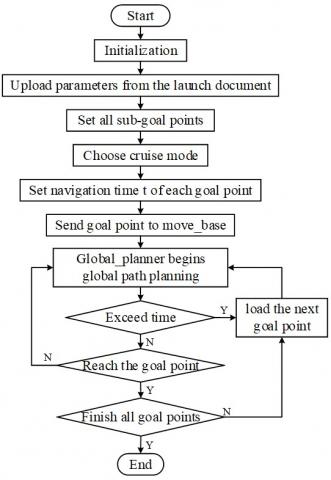
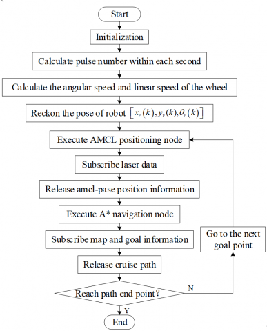
Using the two-dimensional environment map established based on the Gmapping algorithm, the global path planning based on the A* algorithm could only find an optimal cruise path between the initial point and the goal point, and it cannot perform a traversal cruise over all plants in accordance with the characteristics of “row planting”. Therefore, according to the operational requirements, we set a series of goal points on the map as the track of the path cruise. After the PC supervision terminal releases the cruise order, the robot would reach the first goal point, and after the actuator completes its operation within the working range, that point would become the initial point. In relying on the A* algorithm, the robot would continue to seek the optimal path to the next goal point, and in this way, the initial point and the goal point would be updated continuously, and ultimately, the specific path cruise would be completed. The control procedure for the specific path cruise of the greenhouse robot is shown in Figure 12. During the cruise process, the AMCL algorithm is used by the robot to determine its own position, and the DWA algorithm is applied for the dynamic avoidance of debris, plants and pedestrians on the cruise path.
Using the ROS operating system in this article, the global path planning plug-in Global_planner is employed to configure the robot’s path planning document. Considering the working space of the actuator, appropriate stop spacing would be selected, the positions of goal points on the cruise path of the robot would be set on the constructed map, and the greenhouse robot would cruise row by row in an “S”-shaped path along the center aisle.
Figure 12. Working procedures of specific path cruise
2.6 Main program design
Ubuntu 16.04 would be installed in the industrial computer, the ROS system would be configured, and then the chassis controller would be connected through the USB interface. The odometer and lidar are connected carefully. In the ROS system, the four packages, namely, mybot_bringup, rplidar_ros, mybot_description and mybot_navigation, are applied to oversee the chassis driving of the greenhouse robot, the radar driving, description of the robot structure, and the implementation of SLAM and navigation tasks, respectively, and then the navigation positioning system of the greenhouse robot would be designed. Using the Wi-Fi provided by routers, the same static IP address would be allocated to the PC terminal and the industrial computer, and the industrial computer would be remotely supervised by PuTTY software at the PC terminal to obtain the real-time state of the greenhouse robot during the autonomous operation process.
Figure 13. Odometer reckoning procedure chart
The primary program procedure of the robot navigation positioning is shown in Figure 13. At first, the PC supervision terminal would release the map composition task, the industrial computer would receive the odometer information sent by the chassis controller and lidar scanning data, and the two-dimensional map would be established. Then, a new scritcps folder would be created in the/ROS/mybot0323/mybot_navigation of the ROS working space, and then the programing of the cruise node would be performed. Based on the constructed map and according to the working demand of the robot, all the goal points would be set. Furthermore, the PC supervision terminal would release the cruise task, and the chassis controller of the robot would read encoder pulse number N1 after every sampling period ∆t. The pulse number output obtained by the encoder every second is N2=N1/∆t, and then the angular speed and linear speed of the wheel could be calculated. According to the odometer model, the robot pose at the current moment is Xr=[xr(k), yr(k), θr(k)]. The chassis controller of the robot would then send the pose information to the industrial computer through the serial port and receive the motion control order from the industrial computer. Simultaneously, the industrial computer would execute the AMCL positioning node and release the position of the robot combined with the pose information and lidar scanning data. Then, relying on the A*navigation node, the robot would complete its specific path cruise according to the set path.
While working in the greenhouse, the positioning precision while walking in a straight line between planting rows would influence the single operation precision of the greenhouse robot. In addition, the cruise precision of the robot on a specific path would influence the autonomous working continuity of the greenhouse robot. At present, the average deviation of the navigation positioning precision of the greenhouse robot is less than 10.00 cm, and the mean-square deviation is within 2.67 cm2 [21-25]. To test the straight line walking positioning precision and the cruise precision along a specific operating path of the navigation positioning system, the following experiment was performed.
3.1 Positioning precision of straight line walking
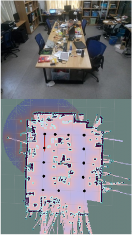
The office area shown in Figure 14 was chosen from Northwest A&F University to test the positioning precision of the integrated odometer/lidar navigation positioning system during straight line walking in the aisle, the chairs and desks were used to simulate plants, and the corridor was used to simulate the aisle. To test whether the walking track of the robot in the aisle is a straight line, a 10.00 m-long line segment was chosen, and after every 1.00 m, a mark point was made. The coordinates of the 10 goal points were set as the coordinates of the 10 marked points.
At first, the map composition order was released from the PC supervision terminal and the Gmapping program was executed in ROS. The two-dimensional environment map of the laboratory was autonomously established, and then 10 goal points were set on the map. Then, the PC supervision terminal would release the cruise order, and the robot would perform a straight-line cruise using the A* navigation algorithm and AMCL positioning algorithm. A total of 200 straight-line walking tests have been conducted, the coordinates where the robot passed each goal points were recorded, and the 200 walking coordinates of each goal point were averaged. After each test, all the robots were placed at the same initial position to avoid the influence of other factors and guarantee the independence of the test. The two-dimensional grid map is shown in Figure 14, and the test results are shown in Table 1.
The positioning precision of the robot during the cruise process could be represented by the average deviation $\bar{X}$ as calculated by equation (10), and the stability of the robot along the track could be represented by the mean-square deviation S2 obtained in equation (11).
$\bar{X}=\frac{1}{N} \sum_{i=1}^{N} X_{i}$ (10)
$S^{2}=\frac{1}{N} \sum_{i=1}^{N}\left(X_{i}-\bar{X}\right)^{2}$ (11)
Therefore, according to the data in Table 1, when the number of goal points is N=10, the average deviation from the track during straight-line walking along the aisle is $\bar{X}$=3.34cm, among which the largest deviation distance is 4.93 cm, and the mean-square deviation during straight-line walking along the aisle is S2 =1.38cm2. At present, it the average deviation of the navigation positioning precision of greenhouse robot shall be less than 10.00 cm, and the mean-square deviation shall be less than 2.67 cm2. The test results show that the navigation positioning precision of that navigation positioning system could satisfy the navigation positioning requirements and the track deviation requirements of the greenhouse robot during its autonomous straight line walk.
Figure 14. Test scene and two-dimensional grid map
Table 1. Test data from straight line walk (Unit: cm)
|
No. |
Goal points |
Real coordinates |
Deviation |
|
1 |
(0.000, 0.00) |
(0.00, 0.00) |
0.00 |
|
2 |
(100.00, 0.00) |
(101.39, -1.16) |
1.81 |
|
3 |
(200.00, 0.00) |
(200.55, -1.55) |
1.64 |
|
4 |
(300.00, 0.00) |
(300.91, -1.64) |
1.87 |
|
5 |
(400.00, 0.00) |
(401.62, -2.32) |
2.82 |
|
6 |
(500.00, 0.00) |
(501.93, -2.81) |
3.40 |
|
7 |
(600.00, 0.00) |
(602.17, -3.27) |
3.92 |
|
8 |
(700.00, 0.00) |
(702.55, -3.19) |
4.08 |
|
9 |
(800.00, 0.00) |
(802.91, -2.92) |
4.12 |
|
10 |
(900.00, 0.00) |
(902.43, -4.16) |
4.81 |
|
11 |
(1000.00, 0.00) |
(1001.71, 4.63) |
4.93 |
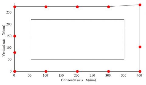
The 10.00 m×8.00 m office area in Northwest A&F University shown in Figure 15 was chosen to test the precision of the integrated odometer/lidar navigation system in a specific path cruise. To test the integrated odometer/lidar navigation system, the desks in the middle and two sides are simulated as ridges, and the corridor is simulated as the aisle, and the aisle width is 1.00 m. The length on the rectangular track is 13.70 m, the 13 points represented by the red points in the map are chosen as the goal points and marked in the site, the interval between each two points is 1.00 m, and the position the greenhouse robot may cover is simulated. The two-dimensional coordinate system with the vertex at the left bottom as the original point is established. The length of the experimental car is 500 mm, the width is 400 mm, and the wheel distance is 300 mm. The set goal points and expected route are shown in Figure 16.
Figure 15. Experimental scene and two-dimensional map of the rectangular path cruise
Figure 16. Goal points and expected route
Table 2. Test data of rectangular path cruise (Unit: cm)
|
No. |
Goal points |
Real coordinates |
Deviation |
|
1 |
(0.00, 0.00) |
(0.00, 0.00) |
0.00 |
|
2 |
(100.00, 0.00) |
(100.61, 1.69) |
1.79 |
|
3 |
(200.00, 0.00) |
(201.46, 2.28) |
2.71 |
|
4 |
(300.00, 0.00) |
(302.08, 2.87) |
3.54 |
|
5 |
(400.00, 0.00) |
(399.52, 2.91) |
2.95 |
|
6 |
(400.00, 104.60) |
(398.07, 102.44) |
2.89 |
|
7 |
(400.00, 283.50) |
(399.54, 284.06) |
0.72 |
|
8 |
(300.00, 275.00) |
(300.11, 280.03) |
5.03 |
|
9 |
(200.00, 275.00) |
(199.51, 277.83) |
2.87 |
|
10 |
(100.00, 275.00) |
(99.59, 275.09) |
0.41 |
|
11 |
(0.00, 275.00) |
(1.34, 275.01) |
1.34 |
|
12 |
(0.00, 150.00) |
(-2.56, 152.07) |
3.29 |
|
13 |
(0.00, 80.00) |
(-2.62, 83.12) |
4.07 |
|
14 |
(0.00, 0.00) |
(-2.78, 2.77) |
3.92 |
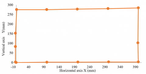
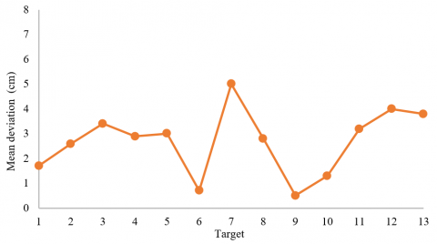
Figure 17. Scatter diagram of specific working path cruise test
Figure 18. Scatter diagram of the mean derivations during the specific working path cruise test
At first, the map composition order would be released from the PC supervision terminal, the Gmapping program would be executed in ROS, and the two-dimensional environment map of the laboratory would be autonomously established. Corresponding to the positions of the points at the site, 13 goal points would be set on the map. Then, the PC supervision terminal would release the cruise order, and the robot would perform a specific path cruise using the A* algorithm. The dynamic avoidance of obstacles on the path was performed through DWA, and the position of the robot at the AMCL time were calculated. A total of 200 specific working path cruise tests have been conducted, the coordinates where each time the robot passing the goal points were recorded, the 200 walking coordinates of each goal point were averaged. After each test, all the robots were placed at the same initial position to avoid the influence of other factors and guarantee the independence of the test. The experimental results are as shown in Table 2, and the scatter diagrams of the specific working path cruise tests for the robot and average deviation are shown in Figures 17 and 18. Figure 17 directly shows that the navigation positioning system could perform a path cruise along the set operation goal points, and it has relatively high navigation positioning precision. Figure 18 calculates the deviation between the ideal positions and practical positions of the 13 goal points, and it quantitatively analyzes the precision of that navigational positioning system.
According to the data in Table 2, when the number of goal points is N=13, equation 10 could be used to show that during the cruise along the regulated working path, the average deviation from the track is $\bar{X}$=2.73cm. The largest deviation distance is 5.03 cm; for the same reason, when the number of goal points is N=13, during the cruise along the regulated working path, the mean-square deviation of the robot is $S^{2}$=1.67cm2. The navigation positioning precision of the greenhouse robot during operation is less than 10.00 cm, which indicates that the positioning precision of the navigation positioning system is relatively high and the robot could perform the precise operation of a regulated working path cruise and satisfy the greenhouse operational requirements. For the same reason, the requested mean-square deviation of the navigation positioning system is smaller than 2.67 cm2, which indicates that the stability of that navigation positioning system is relatively high and the robot could stably perform a cruise along a specific working path.
In conclusion, under the direction of the integrated odometer/lidar navigation positioning system, the average deviation, maximum deviation and mean-square deviation during the operation of the greenhouse robot are all within the requested range of the greenhouse navigation positioning system and could meet the operational requirements of the greenhouse robot.
To solve the problems of the robot’s high-precision specific working path cruise in the greenhouse planting environment, this article presents a robot navigation positioning system based on an odometer/lidar. The Gmapping algorithm and AMCL algorithm are applied to provide map composition and positioning, global path planning is conducted based on the A* algorithm, and finally, according to the characteristic “row planting” and combined with the navigation toolkit in ROS, a specific working path cruise is performed. Through the experiment, it was verified that the navigation positioning system could complete a high precision cruise of a specific working path and meet picking, spraying and fertilizing requirements. In addition, this system has advantages such as a low cost, easy operation and the flexible setting of the cruise path.
During the test of the system, the influence of the ground flatness on the composition of the environment map has not been considered, and thus, this system only applies to autonomous operations on roads with hard surfaces in multispan greenhouse and has poor adaptability to greenhouse roads with gentle slopes on the two sides and irregular obstacles. Therefore, in future research, it will be necessary to establish a three-dimensional dense point cloud and a two-dimensional grid map based on RTAB-MAP of SLAM and a Kinect V2 depth camera to provide a precise map composition of an environment with poor flatness, and to provide precise positioning under that environment, to meet additional requirements of practical greenhouse operations.
This research has received support from the Shaanxi Key Research and Development Program of China (2019NY-171, 2019ZDLNY02-04, 2018TSCXL-NY-05-04). The authors are also gratefully to the reviewers for their helpful comments and recommendations, which make the presentation better.
[1] Li, X.M., Ma, Z.Y., Chu, X., Liu, Y.X. (2019). A cloud-assisted region monitoring strategy of mobile robot in smart greenhouse. Mobile Information Systems, 2019: 5846232. https://doi.org/10.1155/2019/5846232
[2] Ko, M.H., Ryuh, B.S., Kim, K.C., Suprem, A., Mahalik, N.P. (2015). Autonomous greenhouse mobile robot driving strategies from system integration perspective: review and application. IEEE/ASME Transactions on Mechatronics, 20(4): 1705-1716. https://doi.org/10.1109/TMECH.2014.2350433
[3] Jing, Y.P., Liu, G., Xia, Y.X. (2019). Automatic navigation system and control methods based on GNSS-controlled land leveling technology. International Agricultural Engineering Journal, 28(3): 392-399.
[4] Ju, J., Liu, J.Z., Li, N., Li, P.P. (2017). Curb-following detection and navigation of greenhouse vehicle based on arc array of photoelectric switches. Transactions of the Chinese Society of Agricultural Engineering, 33(18): 180-187.
[5] Mahmud, M.S.A., Abidin, M.S.Z., Mohamed, Z., Rahman, M.K.I.A., Iida, M. (2019). Multi-objective path planner for an agricultural mobile robot in a virtual greenhouse environment. Computers and Electronics in Agriculture, 157: 488-499. https://doi.org/10.1016/j.compag.2019.01.016
[6] He, S., Chan, S.H.G. (2016). Wi-Fi fingerprint-based indoor positioning: Recent advances and comparisons. IEEE Communication Surveys and Tutorials, 18(1): 466-490. https://doi.org/10.1109/COMST.2015.2464084
[7] Retscher, G., Tatschl, T. (2017). Indoor positioning using differential Wi-Fi lateration. Journal of Applied Geodesy, 11(4): 249-269. https://doi.org/10.1515/jag-2017-0011
[8] Munguía, R., Nuño, E., Aldana, C., Urzua, S. (2016). A visual-aided inertial navigation and mapping system. International Journal of Advanced Robotic Systems, 13(3). https://doi.org/10.5772/64011
[9] Pershina, J.S., Kazdorf, S.Y., Lopota, A.V. (2019). Methods of mobile robot visual navigation and environment mapping. Optoelectronics, Instrumentation and Data Processing, 55(2): 181-188. https://doi.org/10.3103/S8756699019020109
[10] Du, Z.L., Ma, Y., Li, X.L., Lu, H.M. (2019). Fast scene reconstruction based on improved SLAM. Computers, Materials and Continua, 61(1): 243-254. https://doi.org/10.32604/cmc.2019.05961
[11] Wang, J., Takahashi, Y. (2018). SLAM method based on independent particle filters for landmark mapping and localization for mobile robot based on HF-band RFID system. Journal of Intelligent and Robotic Systems, 92(3-4): 413-433. https://doi.org/10.1007/s10846-017-0701-8
[12] Retscher, G., Hofer, H. (2017). Wi-Fi location fingerprinting using an intelligent checkpoint sequence. Journal of Applied Geodesy, 11(3): 197-205. https://doi.org/10.1515/jag-2016-0030
[13] Wang, G.C., Wang, Q.Y., Sun, Q., Xia, X.W. (2015). A new rotary scheme of the dual-axis rotary inertial navigation system. Journal of Computational and Theoretical Nanoscience, 12(12): 5674-5684. https://doi.org/10.1166/jctn.2015.4702
[14] Luo, H.B., Xu, L.Y., Hui, B., Chang, Z. (2017). Status and prospect of target tracking based on deep learning. Infrared and Laser Engineering, 46(5). https://doi.org/10.3788/IRLA201746.0502002
[15] Bahraini, M.S., Rad, A.B., Bozorg, M. (2019). SLAM in dynamic environments: A deep learning approach for moving object tracking using ML-RANSAC algorithm. Sensors, 19(17): 3699. https://doi.org/10.3390/s19173699
[16] Jiang, Z.T., Zhu, J.H., Lin, Z.Y., Li, Z.Y., Guo, R. (2019). 3D mapping of outdoor environments by scan matching and motion averaging. Neurocomputing, 372: 17-32.
[17] Meng, J., Ren, M.R., Wang, P., Zhang, J.T., Mou, Y.M. (2020). Improving positioning accuracy via map matching algorithm for visual–inertial odometer. Sensors, 20(2): 552. https://doi.org/10.3390/s20020552
[18] Li, L.L., Sun, H.X., Yang, S., Ding, X.W., Wang, J., Jiang, J.L., Pu, X.H., Ren, C.H., Hu, N., Guo, Y.C. (2018). Online calibration and compensation of total odometer error in an integrated system. Measurement: Journal of the International Measurement Confederation, 123: 69-79. https://doi.org/10.1016/j.measurement.2018.03.044
[19] Wang, P., Chen, Z.H., Zhang, Q.B., Sun, J. (2016). A loop closure improvement method of Gmapping for low cost and resolution laser scanner. IFAC-PapersOnLine, 49(12): 168-173. https://doi.org/10.1016/j.ifacol.2016.07.569
[20] Fu, H.H., Xu, J., Zhang, H., Zhang, M., Xu, X.X. (2018). A novel video target tracking method based on lie group manifold. Traitement du Signal, 35(3-4): 331-340. https://doi.org/10.3166/ts.35.331-340
[21] Uyeh, D.D., Ramlan, F.W., Mallipeddi, R., Park, T., Woo, S., Kim, J., Kim, Y., Ha, Y. (2019). Evolutionary greenhouse layout optimization for rapid and safe robot navigation. IEEE Access, 7: 88472-88480. https://doi.org/10.1109/ACCESS.2019.2926566
[22] Li, T.H., Wu, Z.H., Lian, X.K., Hou, J.L., Shi, G.Y., Wang, Q. (2018). Navigation line detection for greenhouse carrier vehicle based on fixed direction Camera. Transactions of the Chinese Society for Agricultural Machinery, 49: 8-13.
[23] Li, L., Zhao, C., Li, C.L., Qin, S.J. (2018). End position detection of industrial robots based on laser tracker. Instrumentation Mesure Métrologie, 18(5): 459-464. https://doi.org/10.18280/i2m.180505
[24] Jia, S.W., Li, J., Qiu, Q., Tang, H.J. (2015). New corridor edge detection and navigation for greenhouse mobile robots based on laser scanner. Transactions of the Chinese Society of Agricultural Engineering, 31(13): 39-45.
[25] Chang, C.L., Song, G.B., Lin, K.M. (2016). Two-stage guidance control scheme for highprecision straight-line navigation of a fourwheeled planting robot in a greenhouse. Transactions of the ASABE, 59(5): 1193-2016.