Chunjun Gao | Dan Qiao* | Xuefu Zhang | Shiyang Liu | Yuanfu Zhou
OPEN ACCESS
This paper aims to disclose the influence of seepage on high slope during the operation phase. Multiple techniques were adopted to disclose how the clogging rate of drain holes affects slope stability, including but not limited to in-situ probe test, close-range photogrammetry, indoor test, and numerical simulation. Firstly, the groundwater was monitored by digital level meter and pore osmometer. The monitoring results show that, when the clogging rate surpassed 80%, the groundwater level in the slope rose by 13m, the porewater pressure grew by 25kPa at the maximum. Next, the rebar stress and anchor cable axial force were measured, revealing that, when the clogging rate surpassed 80%, the shear force on the main rebar of the anti-slide pile increased by 20%, and the axial force of the anchor cable climbed up by 30kN. After that, the slope surface deformation was evaluated by close-range photogrammetry. The evaluation indicates that the surface deformation was 44mm, about 30mm above the alarm value, i.e. the slope faces the risk of instability. Furthermore, the changes in groundwater level and mechanical response of supporting structures were analyzed at different clogging rates, through numerical simulation and finite-element calculation based on strength reduction theory. The numerical results show that: the stress on supporting structures and slope deformation increased linearly, when the clogging rate grew below 60%, while the stress on supporting structures surged up, once the clogging rate exceeded 80%. The finite-element results indicate that, when the clogging rate exceeded 60%, the safety factor of the slope plunged deeply, an evidence of the instability risk. The research results provide new insights into the slope protection in engineering practices.
high slope, in-situ probe test, close-range photogrammetry, numerical simulation, digital level meter, pore osmometer, rebar stress meter and anchor cable axial force meter
Water is a key inducing factor of slope instability. Cao et al. [1] suggested that seepage failure accounts for 88% of the safety accidents in foundation pits and slopes. According to statistics from provinces in southwestern China (e.g. Yunnan, Guizhou and Sichuan), water-related disasters occur more frequently than any other geological disasters in mountainous areas. The situation is particularly serious in slope sections, which take up about 40~55% of mountain roads [2].
Drain holes have been commonly adopted for slope drainage. Previous surveys show that, in the operating phase, the drainage pipelines are often clogged due to the deposition of fine particles, the crystallization and seepage of groundwater, as well as the growth of microbes. As a result, the groundwater level in the slope will rise, posing a serious threat to the stability of the slope and the safety of the supporting structure. During the construction of transport infrastructure in mountainous areas of southwestern China, it is a top priority to ascertain how slope stability is affected by the water accumulated in the slope after the drain holes are clogged. This is both an engineering geological problem and geotechnical problem [3].
Many engineers and scholars have explored the slope instability induced by clogged drain holes. For example, Pedescoll et al. [4], Hua et al. [5], Morvannou et al. [6], Zhao et al. [7], Yu [8], Zhu and Chen [9] analyzed the clogging mechanism of artificial wetlands, and put forward a series of treatment measures. Liu et al. [10] conducted a clogging experiment with an inner inlay helical teeth labyrinth channel irrigation emitter, and determined the sand diameter and content that are most likely to clog the emitter. Using empirical formulas and model tests, Zhou [11] investigated the clogging mechanism of drainage pipes in tunnels caused by groundwater crystallization. Li et al. [12] and Liu et al. [13] conducted drip irrigation experiments to study the clogging law of drippers under different levels of water hardness. Richardson et al. [14] and Garcia and Garcia [15] demonstrated that drainage pipelines could be clogged by factors like organic matter deposition and microbial growth. However, the deep drain holes in high slopes are clogged under the combined effects of multiple factors. It is difficult to fully examine this clogging phenomenon by the above methods. An effective measure is to numerically analyze the seepage field and stress field of the slopes.
Currently, drain holes are mainly simulated by “replacing holes with pipelines” [16], line sink drainage elements [17], drainage substructure [18] and air elements [19]. In previous studies, the function of the drainage hole was often simulated after setting the water head at each point of the hole. In high slope projects, however, the water head varies from drain hole to drain hole, and may be zero at some holes. It is not necessarily reasonable to simulate the drainage effect by assigning a fixed water head. To solve the problem, the “air elements” method can be extended to determine the equivalent permeability coefficient of drainage holes, according to the principle of equivalent head. In other words, each drain hole is treated as a highly permeable medium to simulate its drainage effect. By adjusting the permeability coefficient, it is possible to calculate the stress field and seepage field of each drain hole under different clogging conditions.
Considering the above, this paper aims to further disclose the influence of clogged drain holes on the stability of high slopes. Taking the deep cut slope 2# of Dawangou, China, this paper explores the change of water level in the slope and the mechanical response of the supporting structure, under different conditions, with the aid of in-situ probe test, close-range photogrammetry and numerical simulation. In this way, the influence of clogged drain holes on slope stability was analyzed in a quantitative manner.
In this section, multiple sensors, namely, digital level meter, pore osmometer, rebar stress meter and anchor cable axial force meter, are adopted to measure the change of water level in the slope and the mechanical changes of the supporting structure, laying the basis for slope stability analysis.
2.1 Groundwater level and porewater pressure
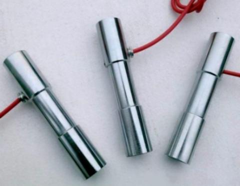
The clogging of drain holes will push up the water level in the slope dramatically, especially on rainy days. In this research, both digital level meter and pore osmometer (Figure 1) were buried in boreholes of Dawangou deep cut slope 2#, and used to capture the changes in groundwater level and porewater pressure (Figures 2 and 3) through the operation phase of the slope.
Figure 1. The pore osmometer
Figure 2. Changes in groundwater level
Figure 3. Changes in porewater pressure
2.2 Forces on anti-slide pile
In the pile-anchor support system, the anti-slide pile is subjected to complex forces, including the lateral earth pressure from the soil behind, the passive earth pressure from the soil in the front, the tension from the anchor cables and its internal force. To identify the forces on the pile at different depths and conditions, ten rebar stress meters (Figure 4) were buried in the slope to measure forces on the pile-soil interface and the free-face. The measured data are presented in Figure 5. Table 1 lists the parameters of the cast-in-situ (CIP) anti-slide pile.
Table 1. The parameters of the cast-in-situ (CIP) anti-slide pile
|
Rebar radius R mm |
Rebar elastic modulus E N/mm2 |
Rebar sectional size S mm2 |
Concrete elastic modulus E N/mm2 |
Concrete sectional size mm2 |
Pile elastic modulus E N/mm2 |
Pile sectional size mm2 |
Fy |
kN |
|
28 |
1.95*105 |
15,393.8 |
2.8*104 |
7.7*105 |
31,371.2 |
7.85*105 |
360 |
221.67 |
Note: The models of rebar and concrete are HRB400 and C30, respectively.
The forces on the pile-soil interface and the free-face can be inversely calculated from the stress on the main rebar of the pile. According to the principle of coordinated deformation, the result of rebar stress meter equals the rebar strain and the pile strain. Hence, the rebar strain $\varepsilon_{g}$ and pile strain $\varepsilon_{z}$ can be respectively computed by:
$\varepsilon_{g}=^{\sigma_{g}} / E_{g}$ (1)
where, $\sigma_{g}$ and $E_{g}$ are the stress and elastic modulus of rebar, respectively.
$\varepsilon_{z}=\sigma_{z} / E_{z}$ (2)
where, $\sigma_{z}$ and $E_{z}$ are the stress and elastic modulus of the pile, respectively.
Figure 4. JMZX-428AT rebar stress meters
Figure 5. The measured data of rebar stress meters
2.3 Forces on anchor cable
The mortar is anchored by its cohesive force and the prestress of the anchor cable, which is transmitted to the soil around the anchor via steel strands. Thus, the elongation of the anchor cable $\Delta L$(mm) can be computed by:
$\Delta L=\frac{P L}{E_{s} A s}$ (3)
where, P is the tensile force (N); L the length of the free section of the prestressed anchor cable (mm); Es is the elastic modulus of the anchor cable (2×10⁵N/mm2); As is the total sectional size of each strand of steel wire (mm2).
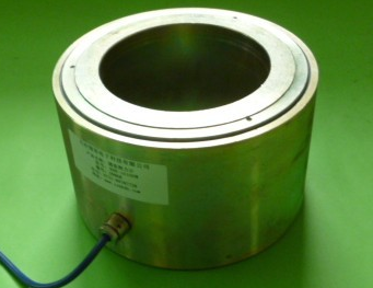
To disclose the forces on the pile at different depths and conditions, two anchor cable axial force meters (Figure 6) were buried to monitor the stress state (Figure 7) of the anchor cable.
Figure 6. JMZX-3320AT anchor cable axial force meter
Figure 7. The measured data of anchor cable axial force meters
2.4 Data analysis
After 8 months of monitoring, the measured data were subjected to statistical analysis. The results show that, when the drain holes were blocked by more than 80%, the groundwater level in the slope rose by 13m, the porewater pressure grew by 25kPa at the maximum, the shear force on the main rebar of the anti-slide pile increased by 20%, and the axial force of the anchor cable climbed up by 30kN.
3.1 Principle of noncontact digital close-range photogrammetry
Following using optical principles, the noncontact digital close-range photogrammetry aims to calculate the 3D coordinates of the target point, according to the image information of the target point, the relevant parameters of the digital camera, and a known point in the same space.
Figure 8. Mathematical principle
The mathematical principle of this approach is explained in Figure 8, where P(X, Y, Z) is a point in space, and $P^{\prime}\left(x_{1}, y_{1}\right)$ and $P^{\prime \prime}\left(x_{2}, y_{2}\right)$ are its projection points on two images; $S\left(X_{S}, Y_{S}, Z_{S}\right)$ is the projection center, i.e. the location of the camera taking the two images; $\omega, \varphi$ and k are the angles between the three axes of the camera coordinate system and those of the coordinate system of point P, respectively; f is the focal length of the camera.
As shown in Figure 8, P, P'(or P'') and S fall on the same straight line. According to the collinearity equation, the relationship between the three points can be expressed as:
$x_{i}=-f \cdot \frac{r_{11}\left(X-X_{S}\right)+r_{12}\left(Y-Y_{S}\right)+r_{13}\left(Z-Z_{S}\right)}{r_{31}\left(X-X_{S}\right)+r_{32}\left(Y-Y_{S}\right)+r_{33}\left(Z-Z_{S}\right)}$ (4)
$y_{i}=-f \cdot \frac{r_{21}\left(X-X_{S}\right)+r_{22}\left(Y-Y_{S}\right)+r_{23}\left(Z-Z_{S}\right)}{r_{31}\left(X-X_{S}\right)+r_{32}\left(Y-Y_{S}\right)+r_{33}\left(Z-Z_{S}\right)}$ (5)
where, i=1, 2; rij can be described as:
$R\left(\omega_{i}, \varphi_{i}, k_{i}\right)=R\left(\omega_{i}\right) R\left(\varphi_{i}\right) R\left(k_{i}\right)=\left[\begin{array}{ccc}{r_{11}} & {r_{12}} & {r_{13}} \\ {r_{21}} & {r_{22}} & {r_{23}} \\ {r_{31}} & {r_{32}} & {r_{33}}\end{array}\right]$ (6)
where,
$R\left(\omega_{i}\right)=\left[\begin{array}{ccc}{1} & {0} & {0} \\ {0} & {\cos \omega_{i}} & {\sin \omega_{i}} \\ {0} & {-\sin \omega_{i}} & {\cos \omega_{i}}\end{array}\right]$
$R\left(\varphi_{i}\right)=\left[\begin{array}{ccc}{\cos \varphi_{i}} & {0} & {-\sin \varphi_{i}} \\ {0} & {1} & {0} \\ {\sin \varphi_{i}} & {0} & {\cos \varphi_{i}}\end{array}\right]$
$R\left(k_{i}\right)=\left[\begin{array}{ccc}{\cos k_{i}} & {\sin k_{i}} & {0} \\ {-\sin k_{i}} & {\cos k_{i}} & {0} \\ {0} & {0} & {1}\end{array}\right]$
Of course, the 3D coordinates of point P cannot be obtained by the collinearity equation alone. Another set of relationships needs to be established. As shown in Figure 3, point P and the two different camera points S' and S'' belong to the same plane. Hence, the coplanarity equation between the three points can be established as:
$F=\left|\begin{array}{lll}{b_{x}} & {b_{y}} & {b_{z}} \\ {u_{1}} & {v_{1}} & {w_{1}} \\ {u_{2}} & {v_{2}} & {w_{2}}\end{array}\right|=0$ (7)
where, $\left[\begin{array}{l}{u_{i}} \\ {v_{i}} \\ {w_{i}}\end{array}\right]=\left[\begin{array}{ccc}{1} & {-k_{i}} & {-\varphi_{i}} \\ {k_{i}} & {1} & {-\omega_{i}} \\ {\varphi_{i}} & {\omega_{i}} & {1}\end{array}\right]\left[\begin{array}{c}{x_{i}} \\ {y_{i}} \\ {-f}\end{array}\right] i=1,2$ and $\left[\begin{array}{l}{b_{x}} \\ {b_{y}} \\ {b_{z}}\end{array}\right]$ is the size of the vector between points S' and S''.
3.2 Analysis of measured displacement
Considering the feasibility, merits and defects of different techniques, the author selected the PhotoModeler Scanner (Eos Systems Inc.) (Figure 9) to process and analyze the measured data, and adopted the FZ-35 camera (Panasonic) and EOS 7D (Cannon) to collect the images (Figure 10).
Figure 9. The interface of PhotoModeler Scanner (PMS)
Figure 10. The cameras
Figures 11-14 show the results of the noncontact close-range photogrammetry on Dawangou deep cut slope 2#.
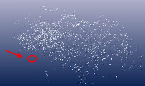
Figure 11. Scatter plot of the slope
Figure 12. Scan model of the slope
Figure 13. Cloud map of the slope
Figure 14. Displacement of scattered points
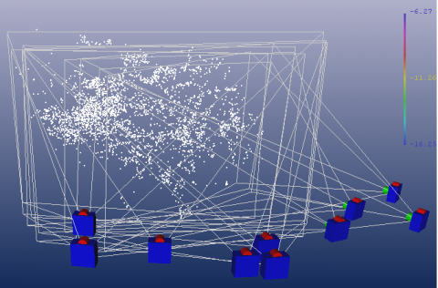
Through the auto-scanning of the images by the PMS, the scattered points were obtained from different positions of the slope. As shown in Figure 14, the scattered points are irregular in distribution, but each point has a fixed number for identification.
In the outdoor test, the straight-line distance between any two points (the red points in Figure 14) was obtained by field measurement, and recorded in the software. On this basis, the distance between any other two points in the figure can be derived according to their relative positions, making it possible to monitor the displacement change of the slope (Figure 15).
Figure 15. The 3D coordinates and distance between any two points
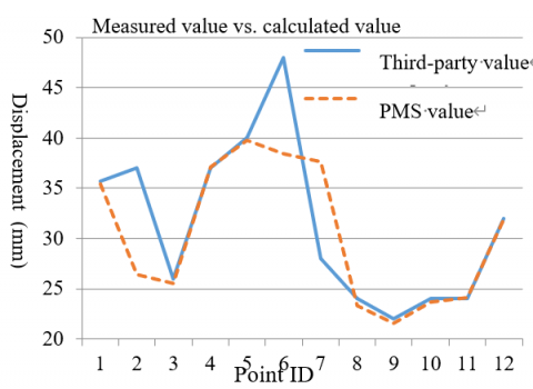
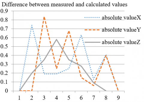
Statistical analysis (Figures 16 and 17) shows that more than 80% of drain holes in the target slope were clogged. The maximum displacement of the slope was 39.78mm, about 30mm above the alarm value. This means the slope faces the risk of instability.
Figure 16. Displacement points on the slope
Figure 17. The measurement errors
Through the analysis, it is confirmed that the noncontact close-range photogrammetry controlled the measurement errors in all directions within 1mm. The measuring accuracy obviously satisfies the technical requirements.
4.1 Prototype parameters and constitutive model
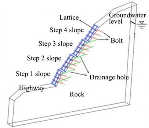
The rock stratum of Dawangou deep cut slope 2# can be divided into two layers: a 1m-thick silty clay layer and a slightly weathered limestone layer. The slope is supported by two methods, namely, a lattice anchor retaining wall and a pile-anchor support system.
The 3D numerical model of the lattice anchor retaining wall (Figure 18) extends 6m along the slope. The size of the model is 100m in length, 6m in width and 77m in height. The rock mass and drain holes were meshed into C3D8RP pore pressure elements, the lattice into C3D8R stress elements, and the anchor rods into T3D2 embedded truss elements.
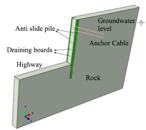
Centering on the anti-slide pile, the 3D numerical model of the pile-anchor support system (Figure 19) extends 60m inside the slope, 50m outside the slope, 30m beneath the pile, and 6m along the slope. The size of the model is 112m in length, 6m in width and 77m in height. The rock mass and drain holes were meshed into C3D8RP pore pressure elements, the anti-slide piles and concrete retaining wall into C3D8R stress elements, and the anchor cables into T3D2 embedded truss elements.
Figure 18. The 3D numerical model of the lattice anchor retaining wall
Figure 19. The 3D numerical model of the pile-anchor support system
The rock stratum of the slope was described by the model based on the Mohr-Coulomb theory of soil strength. This general model of geotechnical mechanics has been successfully applied to simulate the stratum conditions (e.g. soil and rock) in slope support and underground excavation. The model can characterize the engineering mechanics of materials accurately, providing an efficient plastic calculation method. The Mohr-Coulomb model adopts the Mohr-Coulomb criterion and the maximum tensile stress criterion as the failure criteria.
Specifically, the failure envelope $f\left(\sigma_{1}, \sigma_{3}\right)=0$ is defined by the Mohr Coulomb criterion fs=0:
$f^{s}=\sigma_{1}-\sigma_{3} N_{\emptyset}+2 c \sqrt{N_{\emptyset}}$ (8)
From B to C, the failure envelope is defined by the tensile failure criterion ft=0:
$f_{t}=\sigma_{3}-\sigma^{t}$ (9)
where, φ is the friction angle; C is the cohesive force; $\sigma^{t}$ is the tensile strength.
4.2 Simulation parameters and boundary conditions
In Abaqus simulation, the model parameters are given in Table 2 below.
4.3 Simulation conditions
According to the monitored groundwater level and indoor test, the permeability coefficient of the rock and soil of the target slope was set to 0.475m/s. The drain holes were replaced by drain plates for Abaqus simulation (Table 3).
Table 2. Model parameters
|
Material |
Material model |
Density |
Elastic modulus |
Poisson’s ratio |
Saturation permeability coefficient |
Cohesive force |
Friction angle |
|
(kg/m3) |
(GPa) |
(m/s) |
(MPa) |
(°) |
|||
|
Rock mass |
Mohr Coulomb |
2,450 |
0.9 |
0.35 |
4.75E-7 |
4.168 |
35.23 |
|
Drain hole |
Linear elasticity |
1.0 |
0.9 |
0.35 |
4.75E-1 |
- |
- |
|
Drain plate |
Linear elasticity |
2,480 |
0.9 |
0.35 |
3.56E-5 |
0.28 |
30 |
|
Lattice |
Drucker Prager |
2,550 |
28 |
0.3 |
- |
- |
- |
|
Anchor rod |
Linear elasticity |
7,800 |
210 |
0.2 |
- |
- |
- |
|
Anti-slide pile |
Drucker Prager |
2,550 |
28 |
0.3 |
- |
- |
- |
|
Anchor cable |
Linear elasticity |
7,800 |
210 |
0.2 |
- |
- |
- |
Table 3. Simulation conditions
|
Conditions |
Saturation permeability coefficient of drain holes |
Degree of clogging |
Conditions |
Saturation permeability coefficient of drain holes |
Degree of clogging |
|
Condition 1 |
4.75×10⁻¹ |
Normal drainage |
Condition 4 |
4.75×10⁻⁵ |
60% clogged |
|
Condition 2 |
4.75×10⁻³ |
20% clogged |
Condition 5 |
4.75×10⁻⁶ |
80% clogged |
|
Condition 3 |
4.75×10⁻⁴ |
40% clogged |
Condition 6 |
4.75×10⁻⁷ |
100% clogged |
5.1 Comparative analysis on the change of groundwater level
Under each condition, the saturation of each part in the rock mass of the slope was obtained through numerical simulation. The cloud maps of the saturation variation in the lattice anchor retaining wall and the pile-anchor support system are shown in Figures 20 and 21, respectively. Note that the red color stands for full saturation, orange for near saturation, and blue for low saturation. The degree of saturation of the rock mass reflects the groundwater level variation to a certain extent.
The following can be obtained through the comparison between the simulated results and the measured data:
(1) Under the lattice anchor retaining wall, the groundwater level when the drain holes were 40% clogged was nearly 10m higher than that when the drain holes were 20% clogged; the groundwater level increased slowly, after the clogging rate surpassed 60%.
(2) Under pile-anchor support system, the groundwater level first rose slowly with the growth in the clogging rate. Before the clogging rate reached 40%, the groundwater level increased very slightly by less than 1m. Once the clogging rate exceeded 80%, the groundwater level surged up. When the drain holes were fully clogged, the groundwater level climbed up by 13.8m, about twice that at the clogging rate of 80%.
Figure 20. Cloud map of saturation variation in the lattice anchor retaining wall
Figure 21. Cloud map of saturation variation in the pile-anchor support system
5.2 Comparative analysis of forces on supporting structures
The slope failure occurs when the deformation induced by stress field changes exceeds the limit. Here, the slope stability is studied by analyzing the forces on supporting structures. The results of numerical simulation are displayed in Figures 22-25.
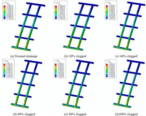
Figure 22. Stress cloud map of the lattice anchor retaining wall
Figure 23. Stress cloud map of the pile-anchor support system
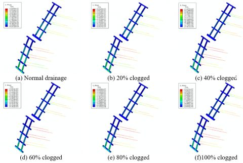
Figure 24. Cloud map of axial force on anchor rods
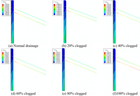
Figure 25. Cloud map of axial force on anchor cables
The above simulation data reflect the change laws of the axial forces on anchor rods and anchor cables at different clogging rates. As shown in Figures 22-25, the axial force on anchor rods remained basically unchanged when the clogging rate was smaller than 80%, and slightly increased when the latter surpassed that level; the axial force on anchor cables increased at an approximately linear rate, when the clogging rate was growing below 60%, had limited changes, when the clogging rate rose from 60 to 80%, and increased further by 10%, after the clogging rate surpassed 80%.
5.3 Comparative analysis of slope stability
Due to the clogging of drain holes, the rock and soil of the slope tend to be saturated, causing a certain reduction in shear strength. To evaluate the slope stability, this paper adopts a reasonable strategy called the strength reduction method. The cohesive force and friction angle of the rock mass were simultaneously reduced for numerical calculation [20, 21]:
$\tau=c^{\prime}+\sigma \tan \varphi^{\prime}$ (10)
where, $c^{\prime}$ and $\varphi^{\prime}$ are the cohesive force and friction angle of the rock mass after the reduction, respectively. The two parameters can be initially calculated as:
$\left\{\begin{array}{l}{c=\frac{c}{F_{s}}} \\ {\tan \varphi^{\prime}=\frac{\tan \varphi}{F_{s}}}\end{array}\right.$ (11)
where, Fs is the reduction factor for the limit equilibrium state, i.e. the safety factor. In numerical calculation, the safety factor is defined as the reduction factor, under which the feature point displacement suddenly changes.
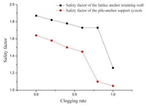
Here, the strength reduction method is used to calculate the safety factor of the slope, and the relationship between the drain hole blocking rate and the slope safety. Taking the displacement change of a node on the top of the slope as the standard, the strength reduction factor at the sudden change of this displacement was taken as the safety factor of the slope. The safety factors of the slope under two supporting structures at different clogging rates were plotted into curves (Figure 26).
Figure 26. Change laws of safety factors of the slope under two supporting structures at different clogging rates
The following can be derived from the curves in Figure 26:
(1) Whichever the clogging rate, the pile-anchor support system achieved a higher safety factor than the lattice anchor retaining wall; with the growth in the clogging rate, the safety factors under two supporting structures both decreased gradually; the decrement was relatively small, when the clogging rate was below 60%.
(2) The safety factors of the slope under both supporting structures plunged deeply, when the clogging rate fell between 60% and 80%.
This paper explores how the clogging rate of drain holes affects slope stability, using in-situ probe test, noncontact close-range photogrammetry, numerical simulation, and finite-element calculation based on strength reduction theory. The main conclusions are as follows:
(1) The groundwater was monitored by digital level meter and pore osmometer. The monitoring results show that, when the clogging rate surpassed 80%, the groundwater level in the slope rose by 13m, the porewater pressure grew by 25kPa at the maximum. According to the monitoring by rebar stress meter and anchor cable axial force meter, when the clogging rate surpassed 80%, the shear force on the main rebar of the anti-slide pile increased by 20%, and the axial force of the anchor cable climbed up by 30kN.
(2) The slope surface deformation was evaluated by close-range photogrammetry. The results show that, the surface deformation was 44mm, about 30mm above the alarm value. This means the slope faces the risk of instability.
(3) The changes in groundwater level and mechanical response of supporting structures were analyzed at different clogging rates, through numerical simulation and finite-element calculation based on strength reduction theory. The numerical results show that: the stress on supporting structures and slope deformation increased linearly, when the clogging rate grew below 60%, while the stress on supporting structures surged up, once the clogging rate exceeded 80%. The finite-element results indicate that, when the clogging rate exceeded 60%, the safety factor of the slope plunged deeply, an evidence of the instability risk. The theoretical, numerical and test results are basically the same.
This work was supported by the National Natural Science Foundation of China (No. 51708070), Chongqing Science and Technology Commission (cstc2017jcyjAX0156, cstc2017shmsA30021, cstc2017jcyjAX0056), Chongqing Municipal Education Commission (KJZH17120), Chongqing Jianzhu College Youth Research Foundation (No.16QK3).
[1] Cao, Q., Li, Q.M., Xiang, W., Jia, H.L. (2012). Automatic monitoring of effects of excavation of group foundation pits on existing adjacent metro tunnels. Chinese Journal of Geotechnical Engineering, 34(S1): 552-556.
[2] Li, J.C. (2005). Study on evaluation method and index of rainfall disaster on highway slope. Chang’an University.
[3] Huang, R.Q. (2008). Geodynamical process and stability control of high rock slope development. Chinese Journal of Rock Mechanics and Engineering, 27(8): 1525-1544. https://doi.org/10.3321/j.issn:1000-6915.2008.08.002
[4] Pedescoll, A., Corzo, A., Álvarez, E., García, J., Puigagut, J. (2011). The effect of primary treatment and flow regime on clogging development in horizontal subsurface flow constructed wetlands: An experimental evaluation. Water Research, 45(12): 3579-3589. https://doi.org/10.1016/j.watres.2011.03.049
[5] Hua, G., Zeng, Y., Zhao, Z., Cheng, K., Chen, G. (2014). Applying a resting operation to alleviate bioclogging in vertical flow constructed wetlands: An experimental lab evaluation. Journal of Environmental Management, 136: 47-53. https://doi.org/10.1016/j.jenvman.2014.01.030
[6] Morvannou, A., Forquet, N., Vanclooster, M., Molle, P. (2013). Characterizing hydraulic properties of filter material of a vertical flow constructed wetland. Ecological Engineering, 60: 325-335. https://doi.org/10.1016/j.ecoleng.2013.06.042
[7] Zhao, W.X., Tao, L., Liu, H.L. (2013). Analysis on clogging mechanism of constructed wetlands and clogging prevention measures. Environmental Science and Management, 38(8): 8-16. https://doi.org/10.3969/j.issn.1673-1212.2013.08.003
[8] Yu, B.H. (2016). Study on the blocking rule and mechanism of constructed wetland. Zhejiang University.
[9] Zhu, J., Chen, H.B. (2009). Discussion on constructed wetlands clogging. China Water & Wastewater, (6): 24-28, 33. https://doi.org/10.3321/j.issn:1000-4602.2009.06.006
[10] Liu, L., Liu, W.Q., Zhou, B. (2012). Influence of sediment particle size on clogging performance of labyrinth path emitters. Transactions of the Chinese Society of Agricultural Engineering, 28(1): 87-93. https://doi.org/10.3969/j.issn.1002-6819.2012.01.017
[11] Zhou, Z. (2015). Study on Mechanism of tunnel drainage pipe blocked by seepage and crystallization of groundwater in karst area and treatment suggestions. Chang’an University.
[12] Li, Y.K., Liu, Y.Z., Li, G.B., Xu, T.W., Liu, H.S., Ren, S.M., Yang, P.L. (2012). Surface topographic characteristics of suspended particulates in reclaimed wastewater and effects on clogging in labyrinth drip irrigation emitters. Irrigation Science, 30(1): 43-56. https://doi.org/10.1007/s00271-010-0257-x
[13] Liu, Y.F., Wu, P.T., Zhu, D.L., Zhang, L., Chen, J.Y. (2015). Effect of water hardness on emitter clogging of drip irrigation. Transactions of the Chinese Society of Agricultural Engineering, 31(20): 95-100. https://doi.org/10.11975/j.issn.1002-6819.2015.20.014
[14] Richardson, J.L., Vepraskas, M.J. (2001). Wetland Soilsgenesis, Hydrology, Landscapes, and Classification. Boca Ratón, FL. CRC Press.
[15] Caselles-Osorio, A., Garcia, J. (2007). Effect of physico-chemical pretreatment on the removal efficiency of horizontal subsurface-flow constructed wetlands. Environmental Pollution, 146(1): 55-63. https://doi.org/10.1016/j.envpol.2006.06.022
[16] Wang, E.Z., Wang, H.T., Deng, X.D. (2001). Pipe to represent hole-Numerical method for simulating single drainage hole in rock-masses. Chinese Journal of Rock Mechanics and Engineering, 20(3): 346-349. https://doi.org/10.3321/j.issn:1000-6915.2001.03.015
[17] Wang, J., Jiang, H.X. (2008). Simulating drainage holes with line sink drainage element. Chinese Journal of Geotechnical Engineering, 30(5): 677-684. https://doi.org/10.3321/j.issn:1000-4548.2008.05.010
[18] Jiang, J.X., Wang, J. (2007). Node mapping method for coacervation degree of freedom for inner nodes in drainage substructure. Water Resources and Power, 25(1): 68-70, 101.
[19] Hu, J., Chen, S.H. (2003). Air element method for modeling drainage holes in seepage analysis. Rock and Soil Mechanics, 2: 281-283, 287. https://doi.org/10.3969/j.issn.1000-7598.2003.02.029
[20] Zhen, Y.R., Zhao, S.Y. (2006). Discussion on safety factors of slope and landslide engineering design. Chinese Journal of Rock Mechanics and Engineering, 25(9): 1937-1940. https://doi.org/10.3321/j.issn:1000-6915.2006.09.032
[21] Ye, H.L., Huang, R.Q., Zhen, Y.R., Du, X.L., Li, A.H. (2010). Sensitivity analysis of parameters for bolts in rock slopes under earthquakes. Chinese Journal of Geotechnical Engineering, 32(9): 1374-1379.