Redouane Mihoub* | Abdelouahab Amroune | Sidi Mohammed El Amine Bekkouche | Rachid Djeffal | Abdelaziz Benkhelifa
OPEN ACCESS
This paper designs a novel estimation model for the temperature of limestone soil, which is abundant in Ghardaia in the Sahara of Algeria. The model was developed based on the radial basis function (RBF), and used to predict soil heat based on two inputs, namely, air temperature and solar radiation. The raw data were collected over more than three years by a meteorological station in the study area. For comparison, the soil temperature was also measured by soil probes arranged at an equal interval. The soil heat predicted by our model based on the raw data were contrasted with the results of field measurement. On this basis, the thermal comfort range of limestone soil for air-conditioning systems was determined. The results show that our model can effectively estimate the temperature of limestone soil in the study area, the thermal comfort range of limestone soil falls between 17.43°C and 29.90°C at the depth of 0.40m, and the temperature near the soil surface (<5m) has seasonal variations.
limestone soil, temperature, solar radiation, estimation
It exists a natural geothermal flux on the surface of the globe, but it is so weak that it can be directly captured. In reality, we exploit the heat accumulated, stored in some parts of the basement. The temperature reached at the surface of underlying formation will be the starting point of the temperature profile through this formation. Low temperature energy available in environments shallow geological (a few tens of meters) can be used by geothermal pumping systems to meet heating and cooling needs Geological materials are favorable environments to the storage of energy since their weak conductivities.
Geological Science is a part of the renewable energy which is to extract the heat stored in the ground for the production of electricity, is geothermal high temperature [1], or heating, geothermal energy at low temperature [2]. The solar field is a set of data describing the evolution of solar radiation available during a given period and its influence on the temperature of the soil. It is used in areas as diverse as agriculture, meteorology and energy applications, and public safety [3]. In the exploitation of solar energy systems, the needs for data of insolation are vitally important both in the design and development of these systems in the assessment of their performance [4]. The optimal temperature is usually obtained at the beginning of season for hot well storage - cold well and end of season in the case of the scanning doublet [5]. Seasonal variations in temperature can particularly affect the temperature of the soil and thus storage [6]. The thermal losses that affect the efficiency of energy storage are mainly due to diffusion in the hanging wall (influence of the proximity of the soil) and to the dispersion hydrodynamics. The existence of a solid and reliable basis is necessary at least the economic survival of the collection and the conversion of solar energy facilities. Although there are networks of stations which are the solar assessment, the number of these stations is very limited. In Algeria, only seven stations are since 1970, the scope of the global element and dissemination of solar radiation [7].
The chemical geothermometry was created to contribute to the appreciation of the temperatures reached in the geothermal reservoirs .During their superficial and / or subterranean course under the effect of temperature, pressure and the possible presence of gas, they react with the constituent minerals of the traversed rocks, which are altered; the water thus acquires its mineralization at the expense of these minerals and, over time, a chemical equilibrium is established which is essentially a function of the temperature reached. The methods of chemical geothermometry allow, from the analysis of the waters, to calculate the temperature to which they were brought in the subsoil "at their level of their deposit". these means of estimating the temperatures in depth called chemical geothermometers [8].
The vapor losses associated with the boiling of the ascending solution either by adiabatic expansion with constant enthalpy for waters emerging with temperatures close to or above the boiling point, in which case the water gives heat to the host rock or by conduction for waters emerging with temperatures below the boiling point; that is to say, the transformation water-vapor is done without heat exchange with the outside because it is all consumed in the phase change [9].
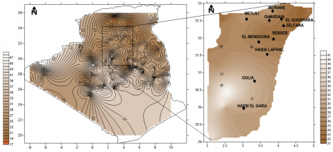
For the moment, the Sahara is well endowed with fossil energy thanks to its deposits of oil and especially gas. It is possible, however, that in certain specific cases other renewable sources of energy may be more cost-effective or more practical to implement. The experimental data used in this paper (solar radiation, temperature, etc.), have been collected at the Applied Research Unit for Renewable Energies, (URAER) situated in the south of Algeria (Figure 1) [10]. Far from the Ghardaïa city with latitude: “+32.370”, longitude “+3.770”, and altitude of “450 m” above the mean level.
The geomorphological in which the M'Zab inscribed is a rocky plateau, of HAMADA; the altitude varies between “300 and 800 meters”. The landscape is characterized by a vast stony expanse where a bare black and brown rock is exposed (Figure 2). This plateau is masked by the strong fluvial erosion at the beginning of the Quaternary which cut into the southern part flat-topped mounds and shaped valleys [11].
Figure 1. Site location of Ghardaia city: a) Algeria, b) Ghardaia
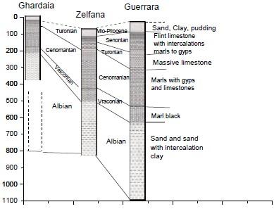
Figure 2. Geology of Ghardaia city
In the perspective of a confrontation with experimental measurements, these are theoretical definitions that were first used. Our models respond satisfactorily to many digital tests. The theoretical model [12, 13], has been used to predict and determine soil temperature by solar radiation and reel temperature by probes temperature soil, respectively. The main objective is to simulate and assess the measurable physical parameters by adjusting the experimental curves with the simulated curves. The results obtained from temperature probes implanted in the soil will inform us about the possibility of exploiting the soil heat to improve the thermal comfort.
The study of the influence of the parameters involved in the variation of the soil temperature characteristics will determine that the air temperature current-carrying phenomenon depends on the solar radiation.
The paper is organized as follow: in the first Section, we present the theory of soil temperature model. In Section two, we deal with Validation model. Results and discussion are given in section three. Finally, the last section was dedicated to the conclusion of the work.
The periodic variations of the radiative flux at the surface which are settled by the general equation of the heat are [14]:
$x C P \frac{d \theta}{d t}=\gamma x \frac{d 2 \theta}{d x 2}+\gamma y \frac{d 2 \theta}{d y 2}+\gamma z \frac{d 2 \theta}{d z 2}+\omega$ (1)
where,
$\theta$: the variation of the soil temperature
$x$: the density
Cp: the specific heat
T: the time
$\lambda x, \lambda y, \lambda z$: The thermal capacity in 3D
$\omega$. represents the heat produced or lost within the Rock (usually $\omega$= 0).
If we consider that the density, the heat capacity and the thermal conductivity are constant and identical in any point of the soil, the equation is written:
$\frac{d \theta}{d t}=\frac{\gamma}{x C p} \frac{d 2 \theta}{d x 2}$ (2)
where,
E: the depth by taking the surface as the origin.
$\frac{\gamma}{\chi C p}$: the thermal diffusivity of the soil. We install $\propto=\frac{\gamma}{x C p}$.
We obtain a particular solution of the equation (1) if it is assumed that the temperature of the soil to infinite depth is equal to the average of the variations of the external temperature.
$\theta(\infty, t)=0$ (3)
This assumption is based on the fact that the temperature of the groundwater at "1 m or 2 m" of depth is very close to the annual average of the temperatures of the air outside [15]. It admits that the temperature of the air at the surface of the soil varies so sine wave, with period T and an amplitude A. at time t1, the temperature of the air will be determined by the equation:
$\theta(0, t 1)=A \cos \left(\frac{2 \pi t 1}{T}\right)$ (4)
At the same time t1, the temperature of the soil to a depth E will be determined by an equation of the following form:
$\theta(E, t 1)=\theta m+A a \cdot \cos (\omega t 1-\emptyset)$ (5)
With
$\omega=\frac{2 \pi}{T}$: pulse of the phenomenon of period t average soil temperature during a
$\theta m$: period of variation (assumed to be the same at all depths)
A: has depreciation of the Amplitude
$\phi$: dephasing phase difference (delay) of the thermal wave
We have seen that $\theta m$ may be assimilated to the annual average of the temperatures of the air. The depreciation and dephasing are given by the following relationships:
$a=\theta . E \sqrt{\frac{\pi}{\alpha T}}$
$\emptyset=E \sqrt{\frac{\pi}{\alpha T}}$
The variations depend on the thermal properties of the soil, of the periodicity of the phenomenon considered and depth.
T: period in hours
a: thermal diffusivity of the soil in m2/h
The dephasing $E \sqrt{\frac{\pi}{\alpha T}}$ Is expressed in radians.
To obtain its value in time, it is necessary to multiply the result by either $\frac{T}{2 \pi}$.
$\emptyset=\frac{T}{2 \pi} \cdot E \sqrt{\frac{\pi}{\alpha T}}-\frac{1}{2} E \sqrt{\frac{T}{\alpha \pi}}$ (6)
The equation of the variation of the temperature in the soil becomes therefore:
$\theta(E, t 1)=\theta m+A a E \sqrt{\frac{\pi}{\alpha t}} \cos \left(\frac{2 \pi}{T} t 1-\frac{1}{2} E \sqrt{\frac{T}{\alpha \pi}}\right)$ (7)
This variation has a wavelength of $2 \sqrt{\pi \alpha T}$
To a depth equivalent to this wavelength, the dephasing is a full period $\phi=\mathrm{T}$ and the temperature is practically stabilized to the annual average of the temperatures of the air outside. This formula allows, when it knows the parameters, to determine the temperature of the soil at different depths for each season, the multiple GPR models due to its simplicity and flexibility identify WEDM-HS process with measurement noise [16].
To simplify the calculations, we are writing the equation of the variation of the temperature in the soil form:
$\theta_{\text {soil}}=\theta m+\sum_{j=1}^{N} A_{T}(j) \cdot\left[\sin \left(\omega(j) T-\emptyset_{T}(j)\right)\right]$ (8)
$\omega=\frac{2 \pi}{T}$
and
$\emptyset_{T}=E \sqrt{\frac{\pi}{\alpha T}}$
$\theta_{\text {soil}}=\theta m+\sum_{j=1}^{N=1061} A_{T}(j) \cdot\left[\sin \left(\frac{2 \pi}{T}(j) t(j)-E \sqrt{\frac{\pi}{\alpha T}}(j)\right)\right]$ (9)
$\theta_{\text {soil}}=\theta m d a y 1+\sum_{j=1}^{N=1} A_{\text {day} 1} \cdot\left[\sin \left(\frac{2 \pi}{T}(\text {day} 1) t(\text {day} 1)-\right.\right.$$E \sqrt{\frac{\pi}{\alpha T}}(d a y 1))]$ (10)
$\theta_{\text {soil}}=\theta m d a y 1061+\sum_{j=1061}^{N=1061} A_{\text {day} 1061}$
$\left[\sin \left(\frac{2 \pi}{T}(d a y 1061) t(d a y 1061)-E \sqrt{\frac{\pi}{\alpha T}}(d a y 1061)\right)\right]$ (11)
$\theta_{\text {soil }}=\theta m d a y 1061+\sum_{j=1061}^{N=1061} A_{\text {day } 1061}$
$\left[\sin \left(\frac{2 \pi}{T}(d a y 1061) t(d a y 1061)-E \sqrt{\frac{\pi}{\alpha T}}(d a y 1061)\right)\right]$ (12)
The equation of the Curve written as:
$y=A \sin \left(P 1\left(\frac{x-x c}{w}\right)\right.$ (13)
where, A=1, w=1.
$y=\sin (P 1(x-x c)$ (14)
We have
∏=3.14
a=8.3910-7 ( diffusivity of soil)
T=8766 h
tday=1061day = 25505.45 h=91819620 second
aT=21399078 10 -9
The final equation of the Curve written as:
$\theta_{\text {soil}}=\theta m d a y 1+$$\sum_{j=1}^{N=1} A_{d a y 1} \cdot\left[\sin \left(\frac{2 \pi}{T}(d a y 1) t(d a y 1)-0 \sqrt{\frac{\pi}{\alpha T}}(d a y 1)\right)\right]$ (15)
$\theta_{\text {soil}}=\theta m d a y 1061+$$\sum_{j=1061}^{N=1061} A_{d a y 1061} \cdot\left[\sin \left(\frac{2 \pi}{T}(d a y 1061) t(d a y 1061)-\right.\right.$$0 \sqrt{\frac{\pi}{\alpha T}}(d a y 1061))]$ (16)
The soil temperature variation equation assumes that the surface temperature can be admitted to the sinusoidal annual variation, and that the earth is a homogeneous medium. In reality, these conditions are never met. Soils are not homogeneous; they are made up of elements of mineral origin and of organic origin, but also of water and air. The thermal characteristics of the soils depend on the nature of their constituents, their respective proportion and their arrangement. More a soil is "airy", the less it will lead the heat and the less it will present of inertia to the warming and cooling (case of the loess for example).
The measures of the soils thermal characteristics are difficult to achieve in situ with the solid probes, hollow, because the temperature gradients cause movements of moisture that distort the results.
The RMSE represent the difference between the predicted values estimated by the model and the measured values. In fact, RMSE identifies the model’s accuracy calculated (Figure 3 and 4).
The performance of RBF models is judged by comparing the estimated values with the measured values using different statistical indexes (Figures 5 and 6) such as Root Mean Square Error “RMSE=0.0029”, Relative Square Error (RRMSE), Determination Coefficient (r2) and Correlation Coefficient “99,05٪”. Mean absolute bias error “MABE=0.0021”.
The heat flow distribution exhibits significant regional variations in general, are related to the local geological structure. The southern area, some relationships with extensional Miocene–Pliocene–Quaternary volcanism suggest an association with recent mantle thermal events.
Evaluation of heat, using temperature measurements (probes temperature soil) and various rock-porosity data reveal an important heat associated with the Algerian Sahara basins (Figure 7). The soil temperatures correlate well with solar energy.
Figure 3. The global solar radiation (GSR)
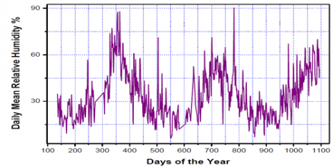
Figure 4. Variation of the humidity
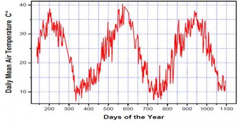
Figure 5. Measured air temperatures
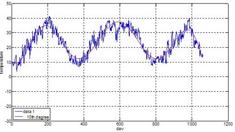
Figure 6. Predicted Soil Temperature based on meteorological data at “E=0 m”
The amplitude of the temperature signal decreases as the depth increases and beyond a distance equal to four times the depth of penetration, the soil temperature stabilizes around the average annual temperature of the surface of the earth ground. Note also that the phase shift is inversely proportional to the thermal diffusivity of the soil (Table 1).
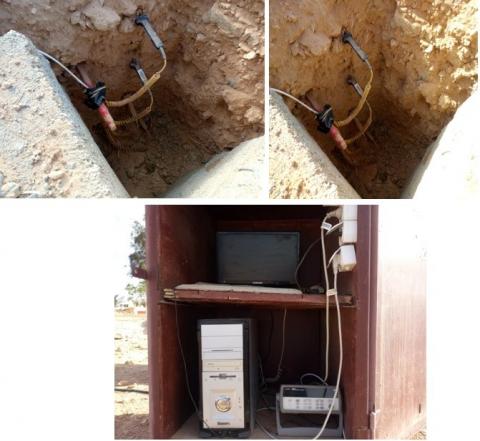
Figure 7. Soil temperature Probes (S1, S2, S3, S4, S5, S6), implanted every “0.20 m”
Table 1. Soil temperature, probes measurements
|
probes |
S1-S2 |
S3-S4 |
S5 |
S6 |
|
temperature |
18°C to 30°C |
32°C to 35°C |
15°C to 28°C |
8°C to 25°C |
The study shows that the penetration depths of the temperature signal take a period of one year greater than one meter for the limestone soil. For thermal comfort we suggest for future uses of hot air, according to the results obtained, all the depth spreads between “0 m and 0.40 m’’, that the temperatures is on average of “35°C’’, is the most ideal for this experimentation and for cold air we suggest the depth of “0.80 m’’ that the temperatures decreases is below “10°C’’ (Figure 8).
Figure 8. Soil Temperature measured ((S1.S2) at “E=0 m”, (S3) at “E= 0.20 m”, (S4) at “E= 0.40 m”, (S5) at “E= 0.60 m”, (S6) at “E=0.80 m”
In order to quantify the energy potential, which is immediately available for direct uses, we have made a preliminary assessment of the heat released by Canadian wells.
The prospects for exploiting this geothermal potential are very encouraging in Ghardaia’s territory. This thermal source makes it possible to develop agriculture under greenhouses (heating greenhouse) and even to heat the premises and homes. In this study, we used: day of the year, day length, average daily temperature, average daily relative humidity, global solar radiation measurements from the Ghardaia City radio station. On the other hand, we have estimated the temperature of the soil, for which soil probes have been inoculated at different depths. The results obtained are very satisfactory because of the strong correlation between the input (air temperature, solar radiation) and the output (soil heat). The examination carried out showed a significant effect of input parameters on the accuracy of soil temperature measurements. It has also been shown that soil temperature evaluated by solar radiation or by RBF models and those measured by probes offer close information and perfect correlations. These results allow us to use the RBF (direct, diffuse) model in areas where probes are not available or in the event of deterioration in reliability measures due to calibration problems that occur after years. The average fluctuation of the temperature at “0.40 m” meter depth is between “17.43 °C and 29.90 °C”; it represents the range of thermal comfort for the case of this study in semi-arid climate. It represents the temperature trapped in the soil all year round. We recommend using more resources from the temperatures of the basement to improve food production, especially the use of greenhouses outside the periods, in this case the climate required in these heated greenhouses to enhance growth. In the perspective of this work, we will study the applicability of this model to different soil types (bare soil and grass soil.
The author would like gratefully acknowledges the Unité de Recherche Appliquée en Energies Renouvelables (Applied Research Unit in Renewable Energies), URAER, Centre de Développement des Energies Renouvelables, CDER, 47133, Ghardaïa, Algeria, For their help and suggestions.
[1] Bastola, H., Peterson, E.W. (2016). Heat tracing to examine seasonal groundwater flow beneath a low-gradient stream in rural central Illinois, USA. Hydrogeology Journal, 24(1): 181-194. https://doi.org/10.1007/s10040-015-1320-8
[2] Shamshirband, S., Mohammadi, K., Chen, H., Samy, G.N., Petković, D., Ma, C. (2015). Daily global solar radiation prediction from air temperatures using kernel extreme learning machine: A case study for Iran. Journal of Atmospheric and Solar- Terrestrial Physics, 134: 109-117. https://doi.org/10.1016/j.jastp.2015.09.014
[3] Kusuda, T., Achenbach, P.R. (1965). Earth temperature and thermal diffusivity at selected stations in the United States (No. NBS-8972). National Bureau of Standards Gaithersburg MD.
[4] Chen, J.L., Li, G.S., Wu, S.J. (2013). Assessing the potential of support vector machine for estimating daily solar radiation using sunshine duration. Energy Conversion and Management, 75: 311-318. https://doi.org/10.1016/j.enconman.2013.06.034
[5] Molz, F.J., Parr, A.D., Andersen, P.F., Lucido, V.D., Warman, J.C. (1979). Thermal energy storage in a confined aquifer: Experimental results. Water Resources Research, 15: 1509-1514. https://doi.org/10.1029/WR015i006p01509
[6] Voigt, H.D., Haefner, F. (1987). Heat transfer in aquifer with finite caprock thickness during a thermal injection process. Water Resources Research, 23: 2286-2292. https://doi.org/10.1029/WR023i012p02286
[7] Guermoui, M., Mekhalfi, M.L., Ferroudji, K. (2013). Heart sounds analysis using wavelets responses and support vector machines. 2013 8th International Workshop on Systems, Signal Processing and their Applications (WoSSPA), pp. 233-238. https://doi.org/10.1109/WoSSPA.2013.6602368
[8] Guendouz, A. (1985). Contribution to the geochemical and isotopic study of the deep aquifers of Sahara northeastern north (Algeria). Postgraduate Thesis Presented at the University of Paris -South, p. 243.
[9] Fournier, R.O., Truesdell, A.H. (1973). An empirical Na, K, Cageothermometer fornatural waters. Geochimicae tCosmochimica Acta, 37(5): 1255-1275. https://doi.org/10.1016/0016-7037(73)90060-4
[10] Şenkal. O., Kuleli, T. (2009). Estimation of solar radiation over Turkey using artificial neural network and satellite data. Applied Energy, 86(7): 1222-1228. https://doi.org/10.1016/j.apenergy.2008.06.003
[11] Fabre, J. (1976). Introduction to the geology of the Algerian Sahara and neighboring regions. Soc. Nat. Ed. SNED, Algiers, p. 142.
[12] Suykens, J.A., Vandewalle, J. (1999). Least squares support vector machine classifiers. Neural Processing Letters, 9(3): 293-300. https://doi.org/10.1023/A:101862860
[13] Wang, J., Bras, R.L. (1999). Ground heat flux estimated from surface soil temperature. Journal of Hydrology, 216(3-4): 214-226. https://doi.org/10.1016/S0022-1694(99)00008-6
[14] Chabert, F. (1980). Thermal environment of semi-buried structures. Excerpt from Frédéric Chabert's thesis "Habitat buried". Educational Pedagogical Unit ABC Group.
[15] Gringarten, A.C., Landel, PA, Menjoz, A., Sauty, J.P (1979). Long-term groundwater storage of low-calorie calories for habitat. Office of Geological and Mining Research, Report No. 79 SGN 683 HYD, Orleans.
[16] Yuan, J., Wang, K., Yu, T., Fang, M.L. (2008). Reliable multi-objective optimization of high-speed WEDM process based on Gaussian process regression. International Journal of Machine Tools and Manufacture, 48(1): 47-60. https://doi.org/10.1016/j.ijmachtools.2007.07.011