Suping Yu | Shangsen Yang* | Wenqing Chen | Weiwei Mao
OPEN ACCESS
The density and depth of grain pile directly affect the evaluation of silo storage. However, there is no report on the detection of mean density of grain pile. To make up for this gap, this paper establishes the relationship between density and dielectric constant through free space transmission method, offering a feasible way to detect the mean density of grain pile. Considering the popularity of ground penetration radar (GPR) in silo detection, the author derived the formula of maximum detection depth, based on the special environment of the silo, the detection quality factor of the radar, and the features of the scattering cross-section. After that, the proposed method was applied to compute the density and depth of grain piles in actual silos. Finally, our method was proved to be accurate through simulation and experiments. The research findings shed new light on the electromagnetic detection of the density and depth of grain pile in actual silos.
finite difference time domain (FDTD), ground penetration radar (GPR), grain pile density; dielectric constant, free space transmission
The safety of food storage is vital to the national well-being and people’s livelihood. To maintain the security of each grain silo, it is necessary to accurately estimate the volume of grain storage, which requires accurate detection of foreign bodies and calculation of grain layer density. In recent years, the ground penetrating radar (GPR) has been widely adopted for grain silo detection, thanks to the strong penetrability and convenience of radar waves [1, 2].
Wave velocity estimation is the key to the GPR-based detection. Currently, the wave velocity can be determined in various ways, such as common midpoint (CMP) method and metal plate reflection method [3]. The wave velocity can be used to derive the dielectric constant. Once the dielectric constant is determined, its correlation with density can be obtained through experiments. The experiments are generally implemented in three steps: Changing the grain pile density multiple times, measuring the corresponding dielectric constants, and fitting the variation laws of the two factors. The above method requires the silo to be regular in shape and proper in size. If the silo is irregular, it would be hard to calibrate the volume after density change. If the silo is too large, the density change cannot occur uniformly. The free space transmission method [4, 5] provides a remote sensing strategy to measure the dielectric constant of grains in a regular, small silo.
In this paper, the free space transmission method is adopted to determine the relationship between dielectric constant and grain pile density in grain silos. Next, the mean dielectric constant of grain silo was derived from the estimated wave velocity of the GPR, and substituted into the relationship model to deduce the mean grain pile density. In addition, the maximum detection depth of the GPR was formulated based on the special environment of the silo, the detection quality factor of the radar, and the features of the scattering cross-section, and verified through experiments. Finally, the density and depth of the target grain silo were computed and confirmed through experiments.
2.1 Wave velocity estimation in shallow round silos
Different categories of silos differ greatly in the height of grain pile. The height is between 10 and 20m for shallow round silos and between 30 and 60m for tower silos. The different heights lead to different detection depths for GPR waves. This paper mainly discusses the measurement of mean dielectric constant of the commonly used shallow round silos [6, 7].
In each shallow round silo, there is a metal plate at the bottom. Since the height of the grain pile equals the detection depth, the dielectric constant can be estimated directly from the reflection delay of the bottom metal plate in the depth direction. The estimation method is illustrated in Figure 1 below, where h is the depth of the grain pile and x is the antenna spacing of the GPR, and measure the electromagnetic wave two-way travel time reflected by the bottom metal plates of the n groups, and find the average:
$\Delta \overline{t}=\frac{1}{n} \sum_{i=1}^{n} \Delta t(i)$ (1)
Thus, the mean dielectric constant of the grain can be obtained as:
$\overline{\varepsilon}=(c / v)^{2}=\frac{c^{2} \Delta \overline{t}^{2}}{4 h^{2}+x^{2}}$ (2)
where c is the speed of radar wave in the air.
Figure 1. Wave velocity estimation in shallow round silos
2.2 Finite difference time domain (FDTD)
The FDTD enjoys unique advantages and wide application in numerical simulation of nonuniform media and scattering electromagnetic field with complex structures [8]. Based on Maxwell’s electromagnetic field equations, the FDTD divides the target area into Yee cells, and assigns different electrical parameters to each cell. Next, the radar waves are transmitted and received at different cell positions according to the actual moving path of the radar. After that, the partial differential equations are converted into difference equations for solution. Since the GPR waves are in two-dimensional transverse mode (TM) in silos, the FDTD algorithm can be expressed as the following partial differential equations:
$\left\{\begin{array}{c}{\frac{\partial E_{z}}{\partial y}=-\mu \frac{\partial H_{x}}{\partial t}+\sigma_{m} H_{x}} \\ {\frac{\partial E_{z}}{\partial x}=\mu \frac{\partial H_{y}}{\partial t}+\sigma_{m} H_{y}} \\ {\frac{\partial H_{y}}{\partial x}-\frac{\partial H_{x}}{\partial y}=-\varepsilon \frac{\partial E_{z}}{\partial t}+\sigma E_{z}}\end{array}\right.$ (3)
where Ez is the electric component in Z direction; Hx and Hy are the magnetic components in X and Y directions, respectively; μ is the magnetic permeability; σm is the permeability; ε is the dielectric constant; σ is the conductivity.
The difference equations can be derived from formula (3) through spatiotemporal dispersion of each component and central difference approximation for first-order partial derivatives:
$E_{z}^{n+1}(i, j)=C A(m) \cdot E_{z}^{n}(i, j)+C B(m)\left(\frac{H_{y}^{n+1 / 2}\left(i+\frac{1}{2}, j\right)-H_{y}^{n+1 / 2}\left(i-\frac{1}{2}, j\right)}{\Delta x}-\frac{H_{x}^{n+1 / 2}\left(i, j+\frac{1}{2}\right)-H_{x}^{n+1 / 2}\left(i, j-\frac{1}{2}\right)}{\Delta y}\right)$ (4)
$H_{x}^{n+1 / 2}\left(i, j+\frac{1}{2}\right)=C P(m) \cdot H_{x}^{n-1 / 2}\left(i, j+\frac{1}{2}\right)-C Q(m) \cdot \frac{E_{z}^{n}(i, j)+1-E_{z}^{n}(i, j)}{\Delta y}$ (5)
$H_{y}^{n+1 / 2}\left(i+\frac{1}{2}, j\right)=C P(m) \cdot H_{y}^{n-1 / 2}\left(i+\frac{1}{2}, j\right)+C Q(m) \cdot \frac{E_{z}^{n}(i+1, j)-E_{z}^{n}(i, j)}{\Delta x}$ (6)
$\begin{align} & CA(m)=\frac{\frac{\varepsilon \left( m \right)}{\Delta t}-\frac{\sigma \left( m \right)}{2}}{\frac{\varepsilon \left( m \right)}{\Delta t}+\frac{\sigma \left( m \right)}{2}}, \\ & CB(m)=\frac{1}{\frac{\varepsilon \left( m \right)}{\Delta t}+\frac{\sigma \left( m \right)}{2}}, \\ & CP(m)=\frac{\frac{\mu \left( m \right)}{\Delta t}-\frac{{{\sigma }_{m}}\left( m \right)}{2}}{\frac{\mu \left( m \right)}{\Delta t}+\frac{{{\sigma }_{m}}\left( m \right)}{2}}, \\ & CQ(m)=\frac{1}{\frac{\mu \left( m \right)}{\Delta t}+\frac{{{\sigma }_{m}}\left( m \right)}{2}}. \\\end{align}$
On this basis, the simulation can be implemented in the following steps:
Step 1: Under the known temporal distribution of electrical field E t1=t0=nΔt and the spatial distribution of magenetic field H (n-1/2)•Δt, calculate the values of H in t2=t1+Δt/2;
Step 2: Calculate the values of E in t1=t2+Δt/2;
Step 3: Repeat Steps 1 and 2. The relationship between time step Δt and space steps Δx & Δy should satisfy:
$c\Delta t\le \frac{1}{\sqrt{{{\left( \frac{1}{\Delta x} \right)}^{2}}+{{\left( \frac{1}{\Delta y} \right)}^{2}}}}$ (7)
3.1 Principle of free space transmission method
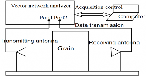
Figure 2 depicts the GPR wave detection system for a grain silo. The grain to be measured is stored in a silo with a fixed volume. The transmitting and receiving antennas are deployed across the grain pile, and connected to their respective ports on the vector network analyzer (VNA). During the detection, the VNA emits and receives the radar waves. The received waves are saved and processed by computer [8]. Let S21 be the transmission coefficient of the GPR waves of the VNA, respectively. Then, the amplitude A and phase Φ of the transmission wave can be obtained as [9]:
$A=-20\log \left| {{S}_{21}} \right|$ (8)
$\Phi =\arg \left( {{S}_{21}} \right)$ (9)
In the free space transmission method, the dielectric constant is determined by computing its real part ε' according to the amplitude A and phase Φ.
Figure 2. The GPR wave detection system
3.2 The real part of dielectric constant
The number of GPR waves in the free space can be expressed as:
${{k}_{0}}=\frac{2\pi }{{{\lambda }_{0}}}$ (rad/m) (10)
where λ0 is the GPR radar wavelength in the air. The number of GPR waves in the medium with a dielectric constant of ε can be computed as:
$k=\frac{2\pi }{{{\lambda }_{0}}}\sqrt{\varepsilon }$ (rad/m) (11)
The phase change induced by the propagation of GPR waves in a medium with a thickness of d can be obtained as:
$\Delta \Phi =\Phi -{{\Phi }_{0}}=kd-{{k}_{0}}d=\frac{2\pi }{{{\lambda }_{0}}}\cdot d\cdot (\sqrt{\varepsilon }-1)$ (12)
Since the grain is a weak conductive medium, we have ε''<<ε'. After eliminating the imaginary part ε'' of the complex dielectric constant, formula (12) can be rewritten as:
${{\varepsilon }^{'}}\approx {{\left( 1+\frac{\Delta \Phi {{\lambda }_{0}}}{2\pi d} \right)}^{2}}$ (13)
Formula (13) is the way to compute the real part of the dielectric constant in the free space transmission method.
3.3 Parameter selection
3.3.1 Measurement frequency
Figure 3. The SWR of the horn antennas
Before the GPR measurement, the measurement frequency should be selected such as to match the antenna frequency. Figure 3 presents the standing wave ratio (SWR) of the horn antennas selected for our experiments. The frequency band of 1~8GHz was selected because the SWR is relatively small in this band.
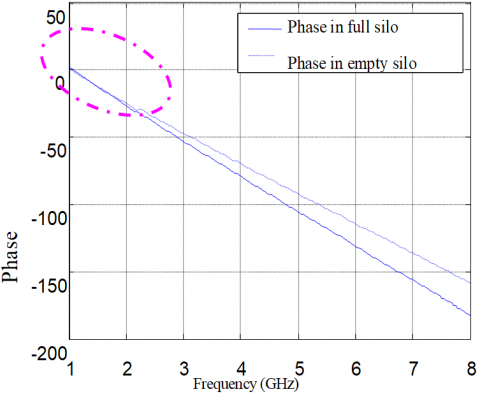
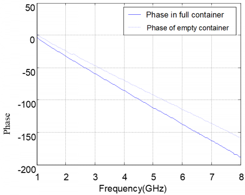
3.3.2 Absolute phase difference
The absolute phase difference should be determined because the phase directly obtained from the measured wave is 2π blurred and entangled in [-π, π]. As shown in Figure 4(a), the phase value measured in the full silo was smaller than that measured in the empty silo, when the frequency fell between 1 and 2GHz. This result clearly goes against the fact. To solve the problem, phase Φ was added to the periodic factor 2πn. Since the silo has a fixed thickness, the n value was selected through trial and error under the constraint of the range of dielectric constraint of the grain [10]. Figure 4(b) provides the results after adding the phase to the periodic factor (2πn, n=1).
(a) Directly extracted phase
(b) Phase added with periodic factors (n=1)
Figure 4. Phase of received waves in free space transmission
4.1 Calculation formula of silo depth
The detection depth of GPR wave depends on various factors, including the electrical property of the medium, the size of the target and the electrical difference between the target and the medium. The quality factor of the GPR detection can be defined as the ratio of the minimum power of the signal received by the receiving antenna to the power of the signal transmitted by the transmitting antenna [11, 12]:
$Q=10\lg \left( \frac{{{\xi }_{T}}{{\xi }_{R}}{{G}_{T}}{{G}_{R}}\cdot g\zeta \cdot {{v}^{2}}\cdot {{e}^{-4\alpha L}}}{64{{\pi }^{3}}{{f}^{2}}{{L}^{4}}} \right)$ (14)
where ξT and ξR are the efficiencies of the transmitting and receiving antennas, respectively; GT and GR are the gains of the transmitting and receiving antennas, respectively; v is the velocity of the GPR wave through the grain layer; g is the backscattering gain of the target; ζ is the scattering cross-sectional area of the target; α is the attenuation coefficient of the medium; L is the distance between transmitting antenna and the target; f for is the center frequency of antennas.
Then, formula (14) can be rewritten as:
$40\lg L+2aL-10\lg \left( \frac{{{v}^{2}}g\zeta }{{{f}^{2}}} \right)=10\lg \left[ \frac{{{\xi }_{T}}{{\xi }_{R}}{{G}_{T}}{{G}_{R}}}{64{{\pi }^{2}}} \right]-Q$ (15)
where a is the attenuation factor of the grain medium:
$a=20\lg {{e}^{\alpha }}=8.68\alpha $ $\left[ {dB}/{m}\; \right]$ (16)
Formula (16) describes how detection depth correlates with GPR performance parameters, target, and medium. It can be seen that the detection depth of the GPR is mainly determined the transmitting power, the antenna gain and the frequency range of the radar system, the dielectric constant of the medium, as well as the scattering cross-section area and scattering gain of the target.
The GPR detection of grain silos needs to extract the actual grain thickness from the detection results. The reflected object in formula (4) is actually the interface between the grain and the silo bottom, which is usually rough cement. The scattering cross-sectional area of such an interface can be empirically determined as the area of the first Fresnel belt. From Figure 5, the maximum propagation length of the GPR wave in the grain can be expressed as:
${{d}_{\max }}=L+{\lambda }/{4}\;$ (17)
where λ is the wavelength of the GPR wave propagating in the grain. The scattering cross-sectional area of the target can be described as:
$\zeta =\pi {{r}^{2}}=\pi \left( \frac{{{\lambda }^{2}}}{16}+\frac{\lambda L}{2} \right)$ (18)
If L>>λ, then ζ can be written as:
$\zeta ={\pi \lambda L}/{2}\;$ (19)
The reflected energy depends on the surface reflectance of the reflector. Thus, the gζ can be described as:
$g\zeta ={\rho \pi \lambda L}/{2}\;$ (20)
where ρ is the power reflection coefficient of the reflecting surface.
Figure 5. Scattering sectional area of rough interface
Inspired by Jiang et al. [13], the relationship model of gζ can be established as:
$g\zeta ={{10}^{{{B}_{1}}}}{{L}^{{{B}_{2}}}}{{f}^{{{B}_{3}}}}$ (21)
where B1=lgπvρ/2; B2=1; B3=1.
Substituting the results into formula (15), the maximum detection depth L of the GPR can be calculated by:
$\lg L+{{D}_{1}}\cdot L={{D}_{2}}$ (22)
$\left\{ \begin{matrix} {{D}_{1}}={2a}/{40-10{{B}_{2}}}\; \\ {{D}_{2}}=\frac{-Q+10\lg \left( {{{\xi }_{T}}{{\xi }_{R}}{{G}_{T}}{{G}_{R}}}/{64{{\pi }^{3}}}\; \right)+10\lg {{v}^{2}}+10({{B}_{1}}+\left( {{B}_{3}}-2 \right)\lg f)}{40-10{{B}_{2}}} \\\end{matrix} \right.$ (23)
where D1 is mainly dependent on the electrical parameters of the medium; D2 is mainly dependent on radar system parameters.
4.2 Simulation of influencing factors on detection depth
To further disclose the impacts of the above factors on detection depth, the author conducted a simulation with the following factors: the antenna gains GT=GR=3, the antenna efficiencies ξT=ξR=1/3, the power reflection coefficient of antenna surfaces ρ=1/3, the real part of the dielectric constant of grain: 4, and the attenuation coefficient: 6dB/m. The above parameters were plugged into formula (23) to obtain different quality factors. The resulting relationship curves between detection frequency and detection depth are displayed in Figure 6. It can be seen that, under a fixed quality factor of the GPR, the detection depth decreased with the increase of detection frequency; under a fixed detection frequency, the effective detection depth increased with the GPR quality factor.
The simulation targets two shallow round silos in China. According to the silo heights, the detection depth should exceed 20m. It can be seen from Figure 6 that the quality factor of the GPR should be no less than 110dB at the transmitting frequency of 0.5GHz, and no less than 90dB at the transmitting frequency of 0.1GHz.
Figure 6. The relationship curves between detection frequency and detection depth
5.1 The relationship between grain pile density and dielectric constant
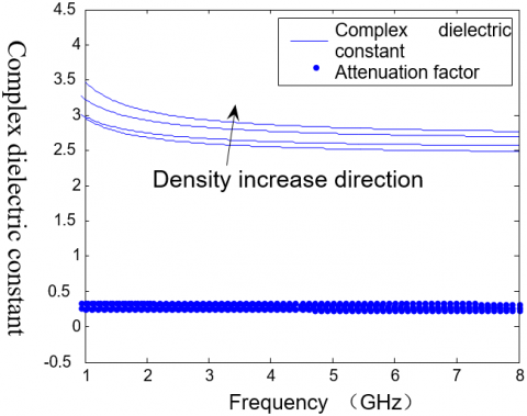
The grain pile density is the overall density of gains and the air between grains in the silo. During our experiments, the sample density was adjusted by adding a fixed amount of grains into the silo to compress the voids between the grains [14]. The silo was simulated by a wooden box with a constant volume. The variations in complex dielectric constant with frequency were monitored under four different grain pile densities and plotted in Figure 7, where the curves are the complex dielectric constant curves fitted from the real and imaginary parts. It can be seen that the real part is sensitive to the change of density, as it increased gradually with the growth in density, while the imaginary part remained basically unchanged despite the change of density.
Figure 7. The relationship between complex dielectric constant and frequency at different densities
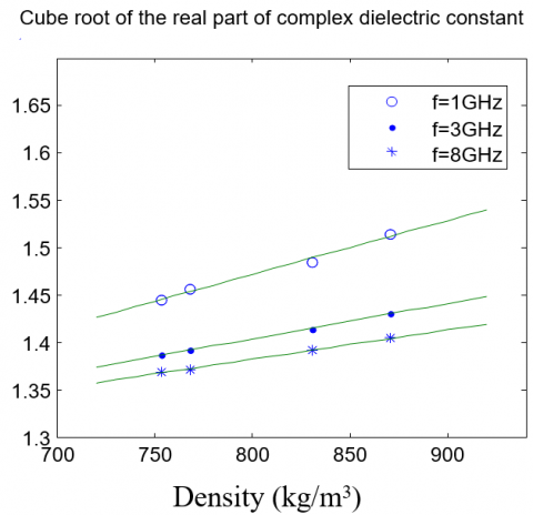
Next, the relationship between the cubic root of the real part of dielectric constant and grain pile density was explored at the frequencies of 1GHz, 3GHz and 8GHz[15], respectively. The results in Figure 8 reveal that the two factors have a linear relationship:
${{\left( {{\varepsilon }^{'}} \right)}^{{}^{1}/{}_{3}}}=k\cdot \rho +b$ (24)
where k, b are constants that varies with frequency.
Figure 8. The relationship between density and dielectric constant
Table 1 lists the values of k and b of the medium in the silo at different detection frequencies. Here, the special case of zero density is adopted for further analysis. In this case, the dielectric constant of the medium equals that of the air. By formula (24), it can be seen that the b values in Table 1, all of which are greater than one, contradicts the reality. This means formula (24) has some limitations and does not apply to compute the medium density whose dielectric constant is close to the air[17].
Table 1. The values of k and b of the medium at different detection frequencies
|
Frequency (GHz) |
k (×10-3) |
b |
|
1 |
0.569 |
1.017 |
|
1.5 |
0.473 |
1.060 |
|
2 |
0.424 |
1.082 |
|
3 |
0.373 |
1.106 |
|
5 |
0.332 |
1.124 |
|
8 |
0.310 |
1.134 |
5.2 Detection depth
Our detection approach was applied in a shallow round silo in Zhuozhou, China. The actual height of the grain pile in the silo is 13m. The parameters of the GPR system were configured as: quality factor=90dB, antenna gain=3dB, antenna efficiency: 1/3, and power reflection coefficient of antenna surface=1/3. The electromagnetic parameters of the grain were directly selected from Section 3.2: the real part of the dielectric constant was 4 and the attenuation coefficient was 6dB/m [10].
The detection depth should be sufficient to cover the actual height of the grain pile and the detection accuracy should be as high as possible. Hence, the rod-shaped GPR antennas with a frequency of 0.3GHz were selected to detect the grain pile height along the radial direction of the silo [11]. The silo length was 25.8m, and the detection was conducted at the step length of 3.5cm. The data were collected from a total of 737 channels, forming the image in Figure 9. It is easy to observe the continuous and stable reflection at the depth of 13m, indicating that the silo bottom is 13m deep. The result agrees well with the actual depth of the silo bottom. The reflections of foreign bodies can also be seen from the figure (the circular areas). The experimental results confirm that the selected GPR parameters and proposed calculation method can achieve accurate detection of grain pile height and locate the foreign bodies in the silo. Suffice it to say that our method lays the technical basis for the extraction of effective target echo [12].
Figure 9. GPR image of the target silo
In light of the features of grain and silos, this paper designs an electromagnetic way to detect grain pile density and height in silos. Firstly, the mean dielectric constant of the target silo was derived from the estimated velocity of the GPR wave. Then, relationship between dielectric constant and density was established by free-space transmission detection method. After that, the mean dielectric constant was substituted into the relationship model to determine the mean grain density. In addition, the proposed method was applied to simulation and experiments on actual silos. The research results show that the GPR detection performance in grain silos depends on the following factors: silo shape [13], actual height of grain pile, the electromagnetic features of grain, reflection surface, antenna parameters, and detection frequency.
The free-space transmission detection method and the proposed relationship model can be applied to measure the properties of other agricultural products with small particle size and determine their density in storage. Of course, the model parameters should be redefined through experiments. The research findings lay a theoretical basis and provide technical support to the selection of the performance parameters of the GPR in silo detection.
The content of this paper is the stage research results of Henan Science and Technology Research Project (182102110099, 162102310474, 172102210400, 172102210395). At the same time, I would like to thank the relevant experts of Henan University of Technology for their technical support.
[1] Thurber, C.H., Ellsworth, W.L. (1980). Rapid solution of ray tracing problems in heterogeneous media. Bulletin of the Seismological Society of America, 70: 1137-1148. https://doi.org/10.1007/BF02245436
[2] Vidale, J. (1988). Finite-difference traveltime calculation. Bulletin of the Seismological Society of American, 78: 2062-2076. https://doi.org/10.1190/1.1442863
[3] Asawaka, E., Kawanaka, T. (1993). Seismic ray tracing using linear travel time interpolation. Geophysical Prospecting, 41(1): 99-111. https://doi.org/10.1111/j.1365-2478.1993.tb00567.x
[4] Moser, T.J. (1991). Shortest path calculation of seismic rays. Geophysics, 56: 59-67. https://doi.org/10.1190/1.1442958
[5] Fischer, R., Lees, J.M. (1993). Shortest path ray tracing with sparse graphs. Geophysics, 58: 987-996. https://doi.org/10.1190/1.1443489
[6] Klimes, L., Kvasnicha, M. (1994). 3-D network ray tracing. Geophysical Journal International, 116(3): 726-738. https://doi.org/10.1111/j.1365-246X.1994.tb03293.x
[7] Guo, M., Zhang, L.N. (2011). Research and development of stored grain insect detection method based on acoustic signal. Journal of the Chinese Cereals and Oils Association, 26(12): 123-128.
[8] Ge, D.B., Yan, Y.B. (2012). The method of electromagnetic finite difference time domain. Xi'an University of Electronic Science and Technology Press, 15-18.
[9] Luo, S.M., Zhou, Z.M. (2012). A review of acoustic detection technology for the stored whea. Journal of the Chinese Cereals and Oils Association, 27(3): 125-128. https://doi.org/10.3969/j.issn.1003-0174.2012.03.027
[10] Tang, L., Chen, M.J. (2016). Image denoising method using the gradient matching pursuit. Mathematical Modelling of Engineering Problemsv, 3(2): 53-56. https://doi.org/10.18280/mmep.030201
[11] Tang, L. (2015). Super-resolution reconstruction method integrated with image registration. Review of Computer Engineering Studies, 2(1): 31-34. https://doi.org/10.18280/rces.020105
[12] Fajardo-Flores, S., Archambault, D. (2014). Evaluation of a prototype of a multimodal interface to work with mathematics. Modelling, Measurement and Control C, 75(2): 106-118.
[13] Jiang, Y.Y., Zhang, Y., Ge, H.Y. (2010) The research of electromagnetic attenuation characteristics in barn. Grain and Oil Processing, (7): 59-61.
[14] Janarthanan, P., Rajkumar, N., Padmanaban, G., Yamini, S. (2014). Performance analysis on graph based information retrieval approaches. Advances in Modelling and Analysis D, 19(1): 1-14.
[15] Xiu, Z.J. (2006). The research of migration and velocity estimation in signal processing of ground penetrating radar. Graduate School of the Chinese Academy of Sciences, 23-25.
[16] Avchar, A., Choudhary, B.S., Budi, G., Sawaiker, U.G. (2018). Effect of rock properties on rippability of laterite in Iron Ore mines of Goa. Mathematical Modelling of Engineering Problems, 5(2): 108-115. https://doi.org/10.18280/mmep.050208
[17] Tirmizi, S.T., Tirmizi, S.R.U.H. (2017). GIS based risk assessment of oil and gas infrastructure in Sindh, Pakista. Environmental and Earth Sciences Research Journal, 4(3): 55-59. https://doi.org/10.18280/eesrj.040301