OPEN ACCESS
In this paper, the fine-grained dynamic frequency modulation algorithm (FGDFMA) was developed based on critical state points (CSPs), aiming to calculate the optimal operating frequency that minimizes the total power consumption of the system. Focusing on the power consumption management of embedded mobile terminals (EMTs), a system-level power consumption model was put forward, integrating the merits of the dynamic power management (DPM) and the dynamic voltage and frequency scaling (DVF S). Then, the CSP-based FGDFMA was developed after analyzing the CSPs in the power consumption model. Through a simulation on the parameters of actual devices, the proposed algorithm was proved more effective than the DPM and the DVFS.
embedded mobile terminals (EMTs), critical state points (CSPs), fine-grained dynamic frequency modulation algorithm (FGDFMA), power management
Embedded mobile terminals (EMTs) (Pedram, 2006) usually integrate such functions as voice communication, audio/video player, internet browser, GPS, games and email. These functions, while enriching the user experience, are extremely power consuming, prosing a huge challenge to the EMTs powered by batteries. Although the battery capacity has quadrupled and even quintupled over the last 30 years, the stacking of batteries is the main method to expand the power supply to the EMTs. This approach pushes up the cost, size and weight of the EMTs, dragging down the mobility and cost-effectiveness of these devices.
The limit on battery capacity calls for the extension of battery life through system-level power management techniques. One of such techniques is the dynamic power management (DPM) (Chede and Kulat, 2008). The DPM can minimize the system power consumption by switching the operating state of each device in light of the changes to its workload. It is mainly responsible for the dynamic management of peripheral devices or processes. Under this technology, the peripheral devices or CPUs, which has been idle for a sufficiently long time, are turned off or put into sleep state (Marzolla and Mirandola, 2013), aiming to reduce the battery consumption. There are three different kinds of DPM strategies for energy consumption optimization, namely timeout DPM, predictive DPM and stochastic DPM. The timeout DPM (Niewiadomska-Szynkiewicz et al., 2014) determines a time limit based on the observed idle time and switch a device to the sleep mode if the device remains idle longer than the time limit. The predictive DPM (Liu et al., 2015) predicts the current idle time length according to certain rules at the beginning. If the predicted value is longer than the switching threshold, the PMC (Firouzi et al., 2012) will be switched to the corresponding sleep mode right away; Otherwise, the PMC will remain in the prepared state. The stochastic DPM (Rizvandi et al., 2011) views the DPM as a stochastic optimization problem, and uses the stochastic decision model to solve the DPM control algorithm.
The dynamic voltage and frequency scaling (DVFS) (Qiu et al., 2012) is another popular power consumption optimization technique. It provides an important means to reduce the power consumption of embedded systems. To balance the task response time (Li et al., 2017) and system power consumption, the DVFS dynamically adjusts the voltage and frequency of the CPU based on the urgency of the system task. The dynamic adjustment is implemented while the system is running, which effectively reduces the CPU’s energy consumption without sacrificing CPU performance. The reduction of system energy consumption is realized at the cost of a longer task execution time, revealing the trade-off between performance and power consumption. The existing DVFS strategies fall into two categories, namely, the DVFS strategy between tasks and the DVFS strategy within a task. The former allocates the CPU time to multiple tasks and adjusts CPU frequency only at the completion of preemptive tasks, while the latter (Firouzi et al., 2012) can adjust the system’s operating frequency when the task is being executed. The recent studies on the DVFS show that, the system’s energy consumption may be negatively affected if the CPU’s operating frequency is below a certain level, and the balance frequency should be calculated from the energy consumptions of off-chip devices and the CPU.
It can be seen from previous research that the DPM and the DVFS provide energy-saving algorithms for different situations of system power consumption. On the one hand, the DVFS can reduce power consumption by lowering the CPU frequency, because the power consumption is positively correlated with voltage and frequency. Nevertheless, the system operating delay will be lengthened at reduced CPU frequency, such that the DPM cannot meet the conditions to switch the operating mode of the system. On the other hand, the system consumes less power as it enters into the sleep mode earlier at increased CPU frequency; however, the frequency increase will push up the power consumption of the CPU during the operation, and lead to extra energy overhead in the transition to the sleep mode (Marowka, 2014). Whereas most of the existing studies analyze the DPM or DVFS separately, this paper attempts to examine the critical switch points of system states through the combination of the DVFS and the DPM. Specifically, a fine-grained dynamic frequency modulation algorithm (FGDFMA) based on critical state points (CSPs) was developed for battery-powered EMTs, with the aim to reduce the system power consumption while ensuring the real-time performance. Simulation results show that the proposed algorithm manages to lower hardware energy consumption, optimize system power utilization and maximize the battery performance in the discharge period.
2.1. System model in one application cycle
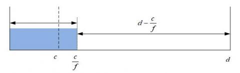
According to the frame-based application model in Figure 1, d is the wake-up period of an application in the embedded real-time system and that application must be completed in any one cycle. The CPU of the model supports the DVFS. Let fmax be the maximum operating frequency of the CPU and c be the worse working time under fmax. Assuming that the application’s execution time varies linearly with frequencies, the worse working time of the application under the operating frequency f can be calculated as:
${{T}_{wcet}}=\frac{c}{f}$ (1)
When f=fmax, the application utilization rate in one cycle d is $U=\frac{c}{d}\le 1$, and the idle time in the cycle is the difference between the application completion time and the next wake-up time. The idle time in one cycle d under the operating frequency f can be calculated as:
$\delta (f)=d-\frac{c}{f}$ (2)
Figure 1. System model in one application cycle
2.2. Device state transition model
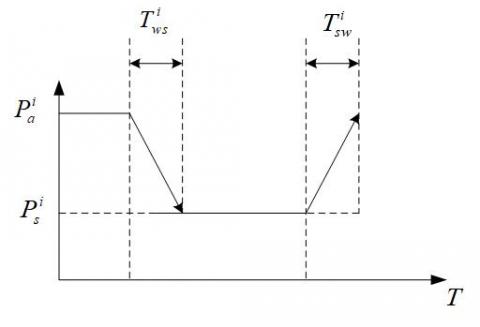
Suppose the embedded real-time system utilizes N devices, denoted as D={D1,D2,...,DN}. Each device is either in the active state or in the sleep state. Let $P_{a}^{i}$, $P_{s}^{i}$, $E_{ws}^{i}$($E_{sw}^{i}$) and $T_{ws}^{i}$($T_{sw}^{i}$) respectively be the power consumption of device i in the active state, the power consumption of device i in the sleep state, the energy consumption of device i as it switches from the active state to the sleep state, and the time of device i to switch from the active state to the sleep state.
Figure 2. State transition overhead
From the start of cycle d, the device should remain active until the application is completed; after the completion, the device can enter the sleep mode to reduce power consumption. However, a certain amount of overhead $E_{ws}^{i}$ is incurred in the state switch of the device. If the idle time δ(f) is too short, the power saved by device i on entering sleep mode will be less than the state switch overhead $E_{ws}^{i}$. Thus, it is necessary to determine the break-even time for the device, that is, the minimum idle time for the state switch. As shown in Figure 2, the break-even time can be expressed as:
${{B}_{i}}=\frac{E_{ov}^{i}-T_{ov}^{i}P_{s}^{i}}{P_{a}^{i}-P_{s}^{i}}$ (3)
where $E_{ov}^{i}=E_{sw}^{i}+E_{ws}^{i}$ is the total consumption of state switch of device i; $T_{ov}^{i}=T_{sw}^{i}+T_{ws}^{i}$ is the total time of state switch of device i. The idle time must surpass the $T_{ov}^{i}$ to make the state switch possible. Thus, we have:
${{B}_{i}}=\max (\frac{E_{ov}^{i}-T_{ov}^{i}P_{s}^{i}}{P_{a}^{i}-P_{s}^{i}},T_{ov}^{i})$ (4)
2.3. Power consumption model
The total power consumption E of the system consists of static power consumption ES and dynamic power consumption E(f):
$E={{E}_{s}}+E(f)$ (5)
The state power consumption ES refers to leakage power, i.e. the minimum power consumption to maintain system operation. In this paper, the total power consumption is realized by reducing the dynamic power consumption E(f) only, considering that the static power consumption can only be eliminated by shutting down the system and that E(f) depends on the system’s operating frequency f.
As shown in Figure 1, assuming that the total number of devices is D, the devices DA={D1,D2,...,Dm} cannot be switched from the active state to the sleep state in a cycle d, if their idle time δ(f)<Bi. Thus, the set of devices that can be switched can be expressed as Di$\in$D-DA. The dynamic power consumption of the system is made up of the power consumption of the CPU, that of all devices D in the non-idle time, that of the devices DA that has not entered the sleep state during the idle time, and the overhead of the state switch:
$E(f)=(a{{f}^{3}}+{{P}_{all}})\frac{c}{f}+\sum\limits_{i|{{D}_{i}}\in {{D}_{A}}}{P_{a}^{i}\times \delta (f)+\sum\limits_{i|{{D}_{i}}\in (D-{{D}_{A}})}{(E_{sw}^{i}+E_{ws}^{i})}}$ (6)
where $a{{f}^{3}}\frac{c}{f}$ is the power consumption of the CPU at the operating frequency f; ${{P}_{all}}\frac{c}{f}$ is the power consumption of all devices during the operating time; $\sum\limits_{i|{{D}_{i}}\in {{D}_{A}}}^{{}}{P_{a}^{i}\times \delta (f)}$ is the power consumption of all devices in the set DA in the idle time; the last term is the power consumption of the state switch of the devices in the set D-DA.
3.1. Determination of the CSPs
The CPU and devices are the main contributors to the total power consumption of the system, which varies with the frequencies. A low frequency may save lots of power through the DVFS, but the prolonged operating time will dampen the DPM effect. Let c be the worst working time of device D0 under fmax, and B0 be the break-even time of the device. Since the task completion time drops from d to c with the growing operating frequency f, the critical frequency for the device D0 to satisfy the break-even time B0 can be obtained by:
${{f}^{*}}=\frac{c}{d-{{B}_{0}}}$ (7)
Hence, device D0 can be switched to the sleep mode as long as the working frequency is greater than f*.
Figure 3. Power consumption functions of the CPU and the device
As shown in Figure 3, taking f* as the critical point, the total power consumption function of the system can be divided into two areas. In area A, the power consumption of the device remains constant at $P_{a}^{i}\times d$ under f<f* because the state switch is impossible. In area B, the operating time $\frac{c}{f}$ of the device decreases linearly with the increase of f; in this case, the power consumption of the device is $\frac{c}{f}\times P_{a}^{i}$. The CPU’s power consumption $a{{f}^{3}}\frac{c}{f}$ always increases with the frequency.
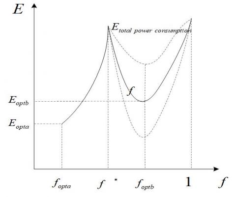
Since Etotal power consumption=Edevice+ECPU, the total power consumption of the system is also a function that changes with f (Figure 4). In interval A, the total power consumption continues to increase because the device power consumption remains unchanged while the CPU consumes more power. In interval B, the CPU power consumption grows while the device power consumption drops with the increase of frequency; if the frequency is below the limit frequency foptb and above f*, the reduction of device power consumption is greater than the increase of CPU power consumption, resulting in a decline of the total power consumption; if the frequency is above the foptb and below the fmax, the reduction of device power consumption is smaller than the increase of CPU power consumption, resulting in a growth of the total power consumption. Therefore, the extreme point foptb of Etotal power consumption falls in the interval [f*, fmax].
Figure 4. Total system power consumption function
3.2. Determination of the optimal frequency
It is easy to find the optimal scheduling point of interval A, but difficult to identify that of interval B. Since all devices in interval B can be switched to the sleep mode after task completion, the power consumption function of interval B can be expressed as:
$E\left( f \right)=\left( a{{f}^{3}}+P_{a}^{0} \right)\frac{c}{f}+\left( E_{\text{sw}}^{0}+E_{ws}^{0} \right)$ (8)
Because E(f) is a strictly convex function and ($E^0_{sd}+E^0_{wu}$) is equivalent to a constant, the extreme point f that can be obtained by taking a derivative of the function:
${{f}_{ee}}={{(\frac{P_{a}^{0}}{2a})}^{1/3}}$ (9)
For any ε>0, E(f) has the following two properties:
Property 1: $\forall f,f>{{f}_{ee}},E\left( {{f}_{ee}} \right)\le E\left( f \right)\le E\left( f+\varepsilon \right)$;
Property 2: $\forall f,f<{{f}_{ee}},E\left( {{f}_{ee}} \right)\le E\left( f \right)\le E\left( f-\varepsilon \right)$.
Then, there are three difference cases for the point of the minimum power consumption in interval B, denoted as fmin:
Case 1: ${{f}^{*}}\le {{f}_{ee}}\le {{f}_{\max }}$
In this case, δ(fee) ≥B0, D0 can be switched to the sleep mode at f=fee, and fee is an extreme point in this interval. Thus, fmin=fee.
Case 2: fee>fmax
According to Property 2, the system consumes the least power at f=fmax in interval B. Thus, fmin=fmax.
Case 3: fee<f*
In this case, δ(fee)<B0 and D0 cannot enter the sleep mode. Thus, fee should approximate f* to make the device suitable for state switch. According to Property 1, the f=f* is the point with the optimal power consumption in interval B under this frequency interval. Thus, fmin=f*.
From the above analysis, we have:
${{f}_{\min }}=\max \left( {{f}^{*}},\min \left( {{f}_{ee}},{{f}_{\max }} \right) \right)$ (10)
3.3. CSP-based FGDFMA
The previous analysis confirms f=U and f=fmin as the points with the optimal power consumption in interval A and interval B, respectively. However, it is still known which of the frequencies has the better optimization effect. To obtain the optimal scheduling algorithm, this section compares the power consumptions between the two intervals.
When the frequency f=fmin and f=U, the CPU power consumption increases by $\Delta {{E}_{\text{c}pu}}=ac\left( f_{\min }^{2}-{{U}^{2}} \right)$, while the device power consumption reduces by:
$\Delta {{E}_{\text{de}vice}}=cP_{\text{a}}^{0}\left( \frac{1}{U}-\frac{1}{{{f}_{\text{min}}}} \right)-{{E}_{t}}$ (11)
The power consumption difference between the CPU and device determines whether the system will be switched to the sleep mode or continue to operate under f=U.
Let ϕ(fmin, U)=△Ecpu-Edevice. If ϕ(fmin, U)<0, then △Ecpu<Edevice. In this case, the optimal scheduling point of the system is fopt=fmin; if ϕ(fmin, U)>0, the optimal scheduling point of the system is fopt=U.
To further display the uncertainty of fopt, the parameters of device Da were configured as c=10, d=42, $P_a^a$=0.5, Esw=Ews=5 and Tsw=Tws=10. Through the above analysis, it can be seen that Ba=20, fee=0.63 and δ(fee)>Ba, indicating that the device can enter the sleep mode. Under these conditions, E(U)=21.57, E(fee)=21.91 and E(U)<E(fee). In this case, the optimal scheduling point of the system is fopt=U. If Esw=Ews=1.25 and Tsw=Tws=5, then E(U)=22.87, E(fee)=22.38 and E(U)> E(fee). In this case, the optimal scheduling point of the system is fopt=fee. Thus, different devices have different fopt.
Through the above analysis, the optimal scheduling algorithm under a fixed system operating frequency can be defined as:
Let ${{f}_{ee}}={{\left( \frac{P_{a}^{0}}{2a} \right)}^{1/3}}$
Let ${{f}^{*}}=\frac{c}{d-{{B}_{0}}}$
fmin=max(f*,min(fee,fmax))
If ϕ(fmin, U)<0, then fopt=fmin; otherwise fopt=U
3.4. Simulation and analysis of the CSP-based FGDFMA
The optimal power scheduling algorithm, i.e. the CSP-based FGDFMA, was simulated with the parameters of actual devices. The maximum operating frequency of the CPU was determined by the ARM CortexA9 chip, the cycle length of the real-time task d was set to 44ms, and the value of B was calculated as 24ms.
If the worst execution time c of the task is longer than 20ms, then the device does not have enough free time to switch to sleep mode. In addition, the system consumes the least power when f=U. Therefore, only the situation c $\in$[2,20] is taken into account.
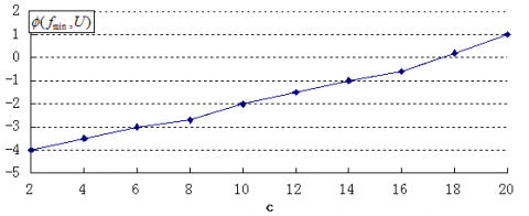
It can be seen from the above analysis that the positivity/negatively of ϕ(fmin, U) depends on the parameters of the device. Through calculation, it is learned that ϕ(fmin, U)<0 when c  [0,18]. In this interval, △Edevice>△ECPU and thus fopt=fmin. ϕ(fmin, U)>0 when c $\in$[18,20]. In this interval, △Edevice<△ECPU and thus fopt=U. The relationship between ϕ(fmin, U) and c is shown in Figure 5 below.
Figure 5. The relationship between ϕ(fmin, U) and c
Here, the proposed algorithm CSP-based FGDFMA is compared with the two popular optimization methods of power consumption below:
-Aggressive slowdown (AG-SD): This algorithm only reduces the power consumption of the CPU, and does not consider the reduction of device power consumption. In this algorithm, the device does not go to sleep, and the operating frequency is always f=U.
-Device-aware slowdown (DA-SD): This algorithm is one of the optimal algorithms for dynamic power adjustment. Unlike CSP-based FGDFMA, the DA-SD fails to consider the DPM and the system power consumption of state switch. By this algorithm, the system will go to sleep if the optimal frequency fee meets the switching condition, and remain active if otherwise.
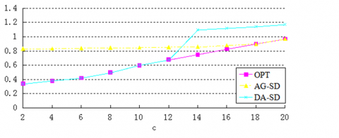
Figure 6. Functional relationships between three different algorithms and c
It can be seen from Figure 6 that, with the growth of the worse working time c, the fopt changed from fee to U. When c<12, the CSP-based FGDFMA selected the DA-SD because ϕ(fmin, U)<0. When c<18, the CSP-based FGDFMA selected the AG-SD because ϕ(fmin, U)>0. When 12<c<18, the CSP-based FGDFMA selected the power consumption function E(f*), which is better than the DA-SD and AG-SD, because fmin=f* and ϕ(f*,U)<0. The simulation results show that the proposed CSP-based FGDFMA outperformed the two contrastive algorithms in power consumption in all intervals.
In this paper, the power consumption management of embedded systems is explored from a new angle. Considering the problems of the DPM and the DVFS and the state switch overhead, the author put forward a system-level power consumption model that integrates the merits of the DPM and the DVFS. After analyzing the CSPs in the power consumption model, the CSP-based FGDFMA was developed to calculate the optimal operating frequency that minimizes the total power consumption of the system. Through a simulation on the parameters of actual devices, the proposed algorithm was proved more effective than the DPM and the DVFS.
This work is supported by the Science and Technology Development Plan of Henan Provincial Department of Science and Technology (Grant No.: 16B510007).
Chede S., Kulat K. (2008). Algorithm to optimize code size and energy consumption in real time embedded system. Journal of Computers, Vol. 3, No. 6, pp. 131-145.
Firouzi F., Azarpeyvand A., Salehi M. E., Fakhraie S. M. (2012). Adaptive fault-tolerant DVFS with dynamic online AVF prediction. Microelectronics Reliability, Vol. 51, No. 6, pp. 1197-1208. http://dx.doi.org/10.1016/j.microrel.2012.01.005
Li F., Liu J. C., Shi H. T., Fu Z. Y. (2017). Multi-objective particle swarm optimization algorithm based on decomposition and differential evolution. Control and Decision, Vol. 32, No. 3, pp. 403-410. Http://dx.chinadoi.cn/10.13195/j.kzyjc.2016.0186
Liu H. B., Liu J. H., He Y. X., Jiang K., Guo C. Y. (2015). Based on the niche particle swarm algorithm of tolerance multi-objective optimization design. Computer integrated manufacturing system, No. 3, pp. 585-592.
Marowka A. (2014). Maximizing energy saving of dual-architecture processors using DVFS. The Journal of Supercomputing, Vol. 68, No. 3, pp. 19-23. https://doi.org/10.1007/s11227-014-1147-4
Marzolla M., Mirandola R. (2013). Dynamic power management for QoS-aware applications. Sustainable Computing: Informatics and Systems, Vol. 3, No. 4, pp. 231-248. https://doi.org/10.1016/j.suscom.2013.02.001
Niewiadomska-Szynkiewicz E., Sikora A., Arabas P., Kamola M., Mincer M., Kołodziej J. (2014). Dynamic power management in energy-aware computer networks and data intensive computing systems. Future Generation Computer Systems, Vol. 37, No. 7, pp. 284-296. https://doi.org/10.1016/j.future.2013.10.002
Pedram M. (2006). Power minimization in embeded system design: Principles and applications. ACM Transactions on Design Automation of Electronics Systems, Vol. 1, No. 1, pp. 3-56.
Qiu M., Ming Z., Li J. Y., Liu S. B., Wang B. (2012). Three-phase time-aware energy minimization with DVFS and unrolling for Chip Multiprocessors. Journal of Systems Architecture, Vol. 58, No. 10, pp. 334-350. https://doi.org/10.1016/j.sysarc.2012.07.001
Rizvandi N. B., Taheri J., Albert Y. (2011). Some observations on optimal frequency selection in DVFS-based energy consumption minimization. Journal of Parallel and Distributed Computing, Vol. 71, No. 8, pp. 1154-1164. http://dx.doi.org/10.1016/j.jpdc.2011.01.004