OPEN ACCESS
In this work Camelopard optimization Algorithm (COA) has been formulated &utilized for solving the optimal reactive power problem. Activities of Camelopard & itsSocial hierarchies are imitated to formulate this algorithm. Normally males use necking, and as a weapon in assaut portion. Among mammals, the tallest living terrestrial animal and it possess the largest ruminants. It has special approach to explore the grass land in quick mode& this aspect has been utilized in the formulation of the algorithm. Efficiency of the projected Camelopard optimization Algorithm (COA) is validated by evaluating in standard IEEE 30, 57, 118, 300 bus test systems. Also by considering the voltage stability evaluation the proposed algorithm has been tested in standard IEEE 30 bus system simulated outcomes shows that genuine power loss has been reduced considerably with variables are in the limits.
optimal reactive power, transmission loss, camelopard optimization algorithm
Real power loss reduction is the main aspect in this problem. Reactive power optimization plays a dominant role in power system operation & control. Reactive power and voltage control are one of the ancillary services to maintain voltage profile through injecting or absorbing reactive power in electricity market (Genco et al., 2018). Various techniques problem (Lee et al., 1984; Deeb and Shahidehpour, 1988; Bjelogrlic et al., 1990; Granville 1994; Grudinin, 1998; Yan et al., 2006) have been utilized but have the complexity in handling constraints. Different types of evolutionary optimization algorithms (Aparajita et al., 2015; Hu et al., 2010; Mahaletchumi et al., 2015; Sulaiman et al., 2015; Pandiarajan et al., 2016; Mahaletchumi et al., 2016; Rebecca et al., 2016; Genco et al., 2017) have been utilized in various stages to solve the problem. But evolutionary algorithms are also stuck into local optimal solution. In this work Camelopard optimization Algorithm (COA) is applied for solving reactive power optimization problem. As herds Camelopards live with related females & offspring, but bachelor herds of adult males are gathered in large aggregations in the grass lands. Social hierarchies are established by males through necking, is used as a weapon in combat bout. Special tactic of searching the grass land in fast mode has been utilized in the formulation of the algorithm. Projected Camelopard optimization Algorithm (COA) efficiency has been verified by testing it in standard IEEE 30, 57, 118,300 bus test systems. Also by considering the voltage stability evaluation the proposed algorithm has been tested in standard IEEE 30 bus system. Simulation output shows that real power loss has been reduced & control variables are within the limits.
Modal analysis for voltage stability evaluation
Power flow equations of the steady state system is given by,
$\left[ \begin{array} { c } { \Delta \mathrm { P } } \\ { \Delta \mathrm { Q } } \end{array} \right] = \left[ \begin{array} { l } { \mathrm { J } _ { \mathrm { p } \theta } \mathrm { J } _ { \mathrm { pv } } } \\ { \mathrm { J } _ { \mathrm { q } \theta } \mathrm { J } _ { \mathrm { QV } } } \end{array} \right] \left[ \begin{array} { l } { \Delta \theta } \\ { \Delta V } \end{array} \right]$ (1)
Where
ΔP = bus real powerchange incrementally.
ΔQ = bus reactive Power injectionchange incrementally.
Δθ = bus voltage angle change incrementally.
ΔV = bus voltage Magnitudechange incrementally.
Jpθ, JPV, JQθ, JQV are sub-matrixes of the System voltage stability in jacobian matrix and both P and Q get affected by this.
Presume ΔP = 0, then equation (1) can be written as:
$\left.\Delta \mathrm { Q } = \left[ \mathrm { J } _ { \mathrm { QV } } - \mathrm { J } _ { \mathrm { Q } \theta } \mathrm { J } _ { \mathrm { P } \mathrm { \theta } ^ { - 1 } } \right] _ { \mathrm { PV } } \right] \Delta \mathrm { V } = \mathrm { J } _ { \mathrm { R } } \Delta \mathrm { V }$ (2)
$\Delta \mathrm { V } = \mathrm { J } ^ { - 1 } - \Delta \mathrm { Q }$ (3)
Where
$\mathrm { J } _ { \mathrm { R } } = \left( \mathrm { J } _ { \mathrm { QV } } - \mathrm { J } _ { \mathrm { Q } \theta } \mathrm { J } _ { \mathrm { P } \theta ^ { - 1 } } \mathrm { JPV } \right)$ (4)
JR denote the reduced Jacobian matrix of the system.
2.1. Modes of voltage instability
Voltage Stability characteristics of the system have been identified through computation of the Eigen values and Eigen vectors.
$\mathrm { J } _ { \mathrm { R } } = \xi \wedge \mathrm { \eta }$ (5)
Where,
ξ denote the right eigenvector matrix of JR, ηdenote the left eigenvector matrix of JR, ∧ denote the diagonal eigenvalue matrix of JR.
$\mathrm { J } _ { \mathrm { R } ^ { - 1 } } = \xi ^ { - 1 } \mathrm { \eta }$ (6)
From the equations (5) and (6),
$\Delta \mathrm { V } = \xi \wedge ^ { - 1 } \eta \Delta \mathrm { Q }$ (7)
or
$\Delta \mathrm { V } = \sum _ { \mathrm { I } } \frac { \mathfrak { \xi} _ { 1 } \eta _ { \mathrm { i } } } { \lambda _ { \mathrm { i } } } \Delta \mathrm { Q }$ (8)
ξi denote the ith column right eigenvector & η is the ith row left eigenvector of JR.
λi indicate the ith Eigen value of JR.
reactive power variation ofthe ith modalis given by,
$\Delta \mathrm { Q } _ { \mathrm { mi } } = \mathrm { K } _ { \mathrm { i } } \xi _ { \mathrm { i } }$ (9)
where,
$\mathrm { K } _ { \mathrm { i } } = \Sigma _ { \mathrm { j } } \xi _ { \mathrm { ij } ^ { 2 } } - 1$ (10)
Whereξji is the jth element of ξi
ith modal voltage variation is mathematically given by,
$\Delta \mathrm { V } _ { \mathrm { mi } } = \left[ 1 / \lambda _ { \mathrm { i } } \right] \Delta \mathrm { Q } _ { \mathrm { mi } }$ (11)
When the value of |λi| =0 then the ith modal voltage will get collapsed.
In equation (8), when ΔQ = ek is assumed ,then ek has all its elements zero except the kth one being 1. Then
can be formulated as follows,$\Delta \mathrm { V } = \sum _ { \mathrm { i } } \frac { \mathrm { n } _ { 1 \mathrm { k } } \xi _ { 1 } } { \lambda _ { 1 } }$ (12)
$\eta_{1k}$ is k th element of $\eta_1$
At bus k V –Q sensitivity is given by,
$\frac { \partial \mathrm { v } _ { \mathrm { K } } } { \partial \mathrm { Q } _ { \mathrm { K } } } = \sum _ { \mathrm { i } } \frac { \eta _ { 1 \mathrm { k } } \xi _ { 1 } } { \lambda _ { 1 } } = \sum _ { \mathrm { i } } \frac { \mathrm { P } _ { \mathrm { ki } } } { \lambda _ { 1 } }$ (13)
Minimization of actual power loss and augmentation of static voltage stability margin index (SVSM) is main key to solve optimal reactive power dispatch problem. Voltage stability evaluation has been done through modal analysis method.
2.2. Minimization of real power loss
Real power loss (Ploss) minimization is given as,
$\mathrm { P } _ { \text {loss } } = \sum _ { \mathrm { k } = ( \mathrm { i } , \mathrm { j } ) } ^ { \mathrm { n } } \mathrm { g } _ { \mathrm { k } \left( \mathrm { V } _ { \mathrm { i } } ^ { 2 } + \mathrm { V } _ { \mathrm { j } } ^ { 2 } - 2 \mathrm { V } _ { \mathrm { i } } \mathrm { V } _ { \mathrm { j } } \cos \theta _ { \mathrm { ij } } \right) }$ (14)
Where n is the number of transmission lines, gk is the conductance of branch k, Vi and Vj are voltage magnitude at bus i and bus j, and θij is the voltage angle difference between bus i and bus j.
2.3. Minimization of voltage deviation
Formula for reducing the voltage deviation magnitudes (VD) is derived as follows,
Minimize $\mathrm { VD } = \sum _ { \mathrm { k } = 1 } ^ { \mathrm { nl } } \left| \mathrm { V } _ { \mathrm { k } } - 1.0 \right|$ (15)
Where nl is the number of load busses and Vk is the voltage magnitude at bus k.
2.4. System constraints
Load flow equality constraints:
$\mathrm { P } _ { \mathrm { Gi } } - \mathrm { P } _ { \mathrm { Di } } - \mathrm { V } _ { \mathrm { i } } \sum _ { \mathrm { j } = 1 } ^ { \mathrm { nb } } \mathrm { v } _ { \mathrm { j } } \left[ \begin{array} { c c } { \mathrm { G } _ { \mathrm { ij } } } & { \cos \theta _ { \mathrm { ij } } } \\ { + \mathrm { B } _ { \mathrm { ij } } } & { \sin \theta _ { \mathrm { ij } } } \end{array} \right] = 0 , \mathrm { i } = 1,2 \ldots , \mathrm { nb }$ (16)
$\mathrm { P } _ { \mathrm { Gi } } - \mathrm { P } _ { \mathrm { Di } } - \mathrm { V } _ { \mathrm { i } } \sum _ { \mathrm { j } = 1 } ^ { \mathrm { nb } } \mathrm { v } _ { \mathrm { j } } \left[ \begin{array} { c c } { \mathrm { G } _ { \mathrm { ij } } } & { \sin \theta _ { \mathrm { ij } } } \\ { + \mathrm { B } _ { \mathrm { ij } } } & { \cos \theta _ { \mathrm { ij } } } \end{array} \right] = 0 , \mathrm { i } = 1,2 \ldots , \mathrm { nb }$ (17)
where, nb is the number of buses, PG and QG are the real and reactive power of the generator, PD and QD are the real and reactive load of the generator, and Gij and Bij are the mutual conductance and susceptance between bus i and bus j.
$\mathrm { V } _ { \mathrm { Gi } } ^ { \min } \leq \mathrm { V } _ { \mathrm { Gi } } \leq \mathrm { V } _ { \mathrm { Gi } } ^ { \max } , \mathrm { i } \in \mathrm { ng }$ (18)
$V _ { \mathrm { Li } } ^ { \min } \leq V _ { \mathrm { Li } } \leq V _ { \mathrm { Li } } ^ { \max } , \mathrm { i } \in \mathrm { nl }$ (19)
$\mathrm { Q } _ { \mathrm { Ci } } ^ { \min } \leq \mathrm { Q } _ { \mathrm { Ci } } \leq \mathrm { Q } _ { \mathrm { Ci } } ^ { \max } , \mathrm { i } \in \mathrm { nc }$ (20)
$\mathrm { Q } _ { \mathrm { Gi } } ^ { \min } \leq \mathrm { Q } _ { \mathrm { Gi } } \leq \mathrm { Q } _ { \mathrm { Gi } } ^ { \max } , \mathrm { i } \in \mathrm { ng }$ (21)
$\mathrm { T } _ { \mathrm { i } } ^ { \mathrm { min } } \leq \mathrm { T } _ { \mathrm { i } } \leq \mathrm { T } _ { \mathrm { i } } ^ { \mathrm { max } } , \mathrm { i } \in \mathrm { nt }$ (22)
$S _ { \mathrm { Li } } ^ { \min } \leq S _ { \mathrm { Li } } ^ { \max } , \mathrm { i } \in \mathrm { nl }$ (23)
As herds Camelopards live with related females & offspring, adult males are in bachelor are in the grass lands in large proposition mode. Social hierarchies are established by males through necking, is used as a weapon in combat bout. Chief distinguishing characteristics are its extremely long neck and legs, its horn-like ossicones, and its distinctive coat patterns. The sole responsibility for raising the young in the herd is by Dominant males.
Special tactic of searching the grass land in fast mode has been utilized in the formulation of the algorithm. In the problem space Camelopard is a 1XNvar array & the array can be defined by,
camelopardfe$= \left[ X _ { 1 } , X _ { 2 } , X _ { 3 } , \ldots , X _ { N _ { v a r } } \right]$ (24)
For each Camelopard the function value can be determined by,
Value $= \mathrm { f } ( \text { Camelopard } ) = \mathrm { f } \left( X _ { 1 } , X _ { 2 } , X _ { 3 } , \ldots , X _ { N a r } \right)$ (25)
Self-regulating nature of Camelopard has been incorporated into the modeled Camelopard optimization Algorithm (COA) & written in Equation (26).
$\mathrm { g } _ { \mathrm { k } + 1 } = \mathrm { g } _ { \mathrm { k } } + \mathrm { r } _ { \mathrm { m } 1 } \mathrm { p } _ { 1 } \left( \mathrm { lo } _ { \mathrm { max } } - \mathrm { n } _ { \mathrm { k } } \right) + \mathrm { r } _ { \mathrm { m } 2 } \mathrm { p } _ { 2 } \left( \mathrm { If } _ { \mathrm { max } } - \mathrm { n } _ { \mathrm { k } } \right)$ (26)
Exploration mentioned by gk, exploitation by nk, learning factors are given by
rm1, rm2, p1, p2 are denoting arbitrary numbers.Lead Camelopard will be act as an interface with abundant Camelopards as indicated in (equation (26)), there will be a comparison between each Camelopard. Movement to various locations by the Camelopard is articulated by following equation,
$\mathrm { n } _ { \mathrm { k } + 1 } = \lambda \left( \mathrm { g } _ { \mathrm { k } } + \mathrm { n } _ { \mathrm { k } } \right)$ (27)
Fitness of each Camelopard will be computed, lqmax(individual Camelopard location), lsmax(best location of the Camelopard herd) will be found. Fitness of the current is better than (lqmax) location vector then that particular value will be saved. Equations (26), (27) utilized to control the movement of the Camelopard. lsmax, lqmaxboth play lead role in the search other & movement to other areas in search is controlled by equation (26). From the maximum vector
is subtracted & it will be multiplied by an arbitrary number , in the range between 0.00, 0.59 by learning parameter rm1, rm2.Camelopard optimization Algorithm (COA)
Step a; Initialization
Step b; In solution space Camelopards are initiated in arbitrary mode
Step c; By using equation (26) fitness values are calculated
Step d; By using equation (27) location of the Camelopards are calculated
Step e; when lsmax updating; if yes next step otherwise goes to step b
Step f; when stop criterion is not met, then go back to step c
Step g; optimized value is output
Camelopard optimization Algorithm (COA) is tested in standard IEEE 30-bus system. In Table 1control variables are given.
Table 1. Limits
|
|
Min Limit |
Max Limit |
|
Generator Bus value |
0.95000 |
1.100 |
|
Load Bus value |
0.95000 |
1.0500 |
|
Transformer-Tap value |
0.9000 |
1.100 |
|
Shunt Reactive Compensator value |
-0.1100 |
0.310 |
Power limits of the generators are listed in table 2.
Table 2. Generators power limits
|
Bus |
Pg |
Pgminimum |
Pgmaximum |
Qgminimum |
Qgmaximum |
|
1 |
96.000 |
49.000 |
200.000 |
0.000 |
10.000 |
|
2 |
79.000 |
18.000 |
79.000 |
-40.000 |
50.000 |
|
5 |
49.000 |
14.000 |
49.000 |
-40.000 |
40.000 |
|
8 |
21.000 |
11.000 |
31.000 |
-10.000 |
40.000 |
|
11 |
21.000 |
11.000 |
28.000 |
-6.000 |
24.000 |
|
13 |
21.000 |
11.000 |
39.000 |
-6.000 |
24.000 |
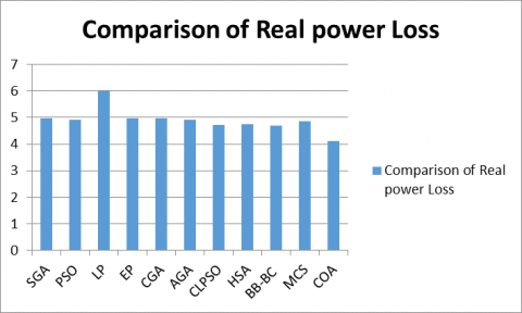
Control variables obtained after optimization given in table 3.COA performance presented in table 4. Comparison of active power loss is given in table 5. Fig 1 gives comparison of real power loss
Table 3. Values of control variable after optimization
|
Parameters |
COA
|
|
Voltage at 1 |
1.041200 |
|
Voltage at 2 |
1.041340 |
|
Voltage at 5 |
1.020720 |
|
Voltage at 8 |
1.030180 |
|
Voltage at 11 |
1.070130 |
|
Voltage at 13 |
1.050420 |
|
T;4,12 |
0.0000 |
|
T;6,9 |
0.0000 |
|
T;6,10 |
0.9000 |
|
T;28,27 |
0.9000 |
|
Q;10 |
0.1000 |
|
Q;24 |
0.1000 |
|
Value of Real power loss (MW) |
4.1024 |
|
Value of Voltage deviation |
0.9080 |
Table 4. COA performance
|
Total number of Iterations |
21 |
|
Total Time taken |
4.97 |
|
Value of Real power loss (MW) |
4.1024 |
Table 5. Evaluation of outcome
|
List of Techniques |
Real power loss (MW) |
|
Method SGA (Wu et al., 1998) |
4.9800 |
|
Method PSO (Zaho et al., 2005) |
4.926200 |
|
Method LP (mahadevan et al., 2010) |
5.98800 |
|
Method EP (mahadevan et al., 2010) |
4.96300 |
|
Method CGA (mahadevan et al., 2010) |
4.98000 |
|
Method AGA (mahadevan et al., 2010) |
4.92600 |
|
Method CLPSO (mahadevan et al., 2010) |
4.720800 |
|
Method HSA (Khazali et al., 2011) |
4.762400 |
|
Method BB-BC (sakthivel et al., 2013) |
4.69000 |
|
Method MCS (Tejaswini et al., 2016) |
4.8723100 |
|
Proposed COA |
4.10240 |
Figure 1. Comparison of real power loss
Table 6. Generator data
|
Generator No |
Pgi minimum |
Pgi maximum |
Qgi minimum |
Qgi maximum |
|
1 |
25.000 |
50.000 |
0.000 |
0.000 |
|
2 |
15.00 |
90.00 |
-17.00 |
50.00 |
|
3 |
10.00 |
500.00 |
-10.00 |
60.00 |
|
4 |
10.00 |
50.00 |
-8.00 |
25.00 |
|
5 |
12.00 |
50.00 |
-140.00 |
200.00 |
|
6 |
10.00 |
360.00 |
-3.00 |
9.00 |
|
7 |
50.00 |
550.00 |
-50.00 |
155.00 |
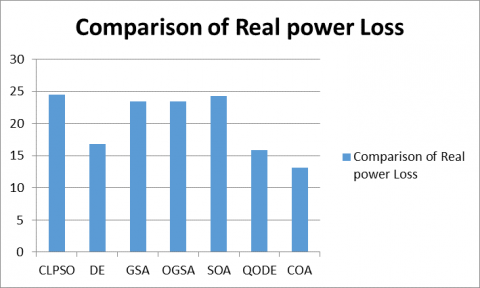
Table 7. Comparison of losses
|
|
Method CLPSO (Dai et al., 2009) |
Method DE (Basu et al., 2016) |
Method GSA (Basu et al., 2016) |
Method OGSA (Shaw et al., 2014) |
Method SOA (Dai et al., 2009) |
Method QODE (Basu et al., 2016) |
COA |
|
PLOSS (MW) |
24.5152 |
16.7857 |
23.4611 |
23.43 |
24.2654 |
15.8473 |
13.086 |
Figure 2. Comparison of loss
Secondly IEEE 57 bus system is used as test system to validate the performance of the proposed algorithm. Total active and reactive power demands in the system are 1247.89 MW and 338.04 MVAR, respectively. Generator data the system is given in Table 6. The optimum loss comparison is presented in Table 7. Fig 2. Gives the comparaison of losses.
Table 8. Reactive power sources limits
|
Bus number |
5 |
34 |
37 |
44 |
45 |
46 |
48 |
|
Maximum value of QC |
0.000 |
14.000 |
0.000 |
10.000 |
10.000 |
10.000 |
15.000 |
|
Minimum value of QC |
-40.000 |
0.000 |
-25.000 |
0.000 |
0.000 |
0.000 |
0.000 |
|
Bus number |
74 |
79 |
82 |
83 |
105 |
107 |
110 |
|
Maximum value of QC |
12.000 |
20.000 |
20.000 |
10.000 |
20.000 |
6.000 |
6.000 |
|
Minimum value of QC |
0.000 |
0.000 |
0.000 |
0.000 |
0.000 |
0.000 |
0.000 |
Table 9. Evaluation of results
|
Active power loss – Minimum & Maximum values |
Methodology - BBO (Cao et al., 2014) |
Methodology - ILSBBO/ strategy1 (Cao et al., 2014) |
Methodology ILSBBO/ Strategy2 (Cao et al., 2014) |
COA |
|
Minimum value |
128.770 |
126.980 |
124.780 |
124.872 |
|
Maximum value |
132.640 |
137.340 |
132.390 |
129.734 |
|
Average value |
130.210 |
130.370 |
129.220 |
126.864 |
Figure 3. Comparison of actual loss
Table 9. shows the comparaison of results.
Then IEEE 118 bus system is used as test system to validate the performance of the proposed algorithm. Table 8 shows limit values.
Finally IEEE 300 bus system is used as test system and Table10 shows the comparaison of real power loss.
With Considering Voltage Stability Evaluation Criterion in IEEE 30 bus system projected algorithm has been verified. Table 11 shows the optimal control variables.
Table 10. Comparison of real power loss
|
Parameter |
Method EGA (Reddy et al., 2014) |
Method EEA (Reddy et al., 2014) |
COA |
|
PLOSS (MW) |
646.2998 |
650.6027 |
629.1898 |
Table 11. COA-ORPD based control variables
|
Parameter |
value |
|
voltage at 1 voltage at 2 voltage at 5 voltage at 8 voltage at 11 voltage at 13 value of T11 value of T12 value of T15 value of T36 value of Qc10 value of Qc12 value of Qc15 value of Qc17 value of Qc20 value of Qc23 value of Qc24 value of Qc29 Real power loss in MW Value of SVSM |
1.03142 1.03418 1.03192 1.02198 1.00032 1.02079 1.00114 1.00021 1.0021 1.0001 3.00 3.00 2.00 0.00 2.00 3.00 3.00 2.00 4.1248 0.2382 |
Static voltage stability index rises from 0.2382 to 0.2396.
In table 12 optimal (control variables) are given.
Figure 4. Comparison of active power loss
Table 12. Value of COA -voltage stability control reactive power dispatch optimal control variables
|
Parameter |
values |
|
voltage at 1 voltage at 2 voltage at 5 voltage at 8 voltage at 11 voltage at 13 value of T11 value of T12 value of T15 value of T36 value of Qc10 value of Qc12 value of Qc15 value of Qc17 value of Qc20 value of Qc23 value of Qc24 value of Qc29 Real power loss in MW Value of SVSM |
1.03279 1.03184 1.03465 1.03254 1.00114 1.03012 0.09001 0.09000 0.09000 0.09000 3.00 3.00 2.00 3.00 0.00 2.00 2.00 3.00 4.9972 0.2396 |
In Table 13 Eigen values are given.
Table 13. Values of settings
|
Area of; Contingency |
ORPD Setting values |
VSCRPD Setting values |
|
28-27 |
0.14100 |
0.14240 |
|
4-12 |
0.16380 |
0.16480 |
|
1-3 |
0.17610 |
0.17720 |
|
2-4 |
0.20220 |
0.20410 |
In table 14 values for limit violation checking has been given with upper & lower limits.
Table 14. Limits of violation
|
Parameter |
Types of Limits values |
Values of; ORPD |
Values of; VSCRPD |
|
|
Lower level |
Upper level |
|||
|
At Q1 |
-20.00 |
151.0 |
1.3421 |
-1.3261 |
|
At Q2 |
-20.00 |
61.00 |
8.9902 |
9.8230 |
|
At Q5 |
-15.00 |
49.920 |
25.926 |
26.000 |
|
At Q8 |
-10.00 |
63.520 |
38.8201 |
40.800 |
|
At Q11 |
-15.00 |
42.0 |
2.9309 |
5.001 |
|
At Q13 |
-15.00 |
48.0 |
8.1020 |
6.030 |
|
At V3 |
0.950 |
1.050 |
1.0371 |
1.0390 |
|
At V4 |
0.950 |
1.050 |
1.0304 |
1.0321 |
|
At V6 |
0.950 |
1.050 |
1.0287 |
1.0290 |
|
At V7 |
0.950 |
1.050 |
1.0100 |
1.0154 |
|
At V9 |
0.950 |
1.050 |
1.0466 |
1.0416 |
|
At V10 |
0.950 |
1.050 |
1.0480 |
1.0492 |
|
At V12 |
0.950 |
1.050 |
1.0402 |
1.0460 |
|
At V14 |
0.950 |
1.050 |
1.0476 |
1.0442 |
|
At V15 |
0.950 |
1.050 |
1.0458 |
1.0412 |
|
At V16 |
0.950 |
1.050 |
1.0420 |
1.0400 |
|
At V17 |
0.950 |
1.050 |
1.0384 |
1.0392 |
|
At V18 |
0.950 |
1.050 |
1.0396 |
1.0402 |
|
At V19 |
0.950 |
1.050 |
1.0382 |
1.0396 |
|
At V20 |
0.950 |
1.050 |
1.0110 |
1.0196 |
|
At V21 |
0.950 |
1.050 |
1.0434 |
1.0248 |
|
At V22 |
0.950 |
1.050 |
1.0446 |
1.0392 |
|
At V23 |
0.950 |
1.050 |
1.0476 |
1.0370 |
|
At V24 |
0.950 |
1.050 |
1.0488 |
1.0374 |
|
At V25 |
0.950 |
1.050 |
1.0140 |
1.0198 |
|
At V26 |
0.950 |
1.050 |
1.0490 |
1.0426 |
|
At V27 |
0.950 |
1.050 |
1.0478 |
1.0458 |
|
At V28 |
0.950 |
1.050 |
1.0246 |
1.0280 |
|
At V29 |
0.950 |
1.050 |
1.0432 |
1.0412 |
|
At V30 |
0.950 |
1.050 |
1.0414 |
1.0390 |
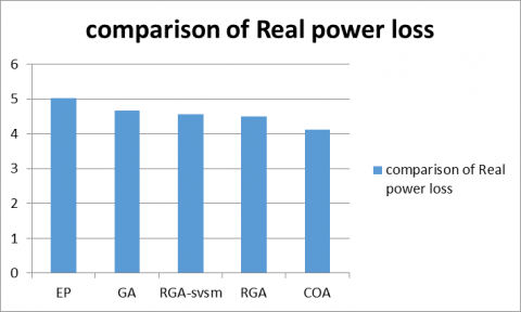
In table 15 over all comparison of real power loss has been given. It indicates that proposed algorithm efficiently reduced power loss. Fig 5. Gives Comparison of real power loss
Table 15. Comparison of losses
|
Technique |
Loss value in MW |
|
Method; Evolutionary programming (Wu et al., 1995) |
5.01590 |
|
Method; Genetic algorithm (Durairaj et al., 2006) |
4.6650 |
|
Method; Real coded GA with Lindex as SVSM (Devaraj et al., 2007) |
4.5680 |
|
Method; Real coded genetic algorithm (Aruna et al., 2010) |
4.50150 |
|
Proposed COA |
4.1248 |
Figure 5. Comparison of real power loss
In this work Camelopard optimization Algorithm (COA) efficiently solved the power problem. Mathematical modeling efficiently improved the search of the optimal solution. Both the exploration & exploitation has been comparatively increased in the proposed technique. Camelopard optimization Algorithm (COA) has performed well when evaluated in standard IEEE 30, 57, 118, 300 bus test systems. Also by considering the voltage stability evaluation the proposed algorithm has been successfully tested in standard IEEE 30 bus system. True power loss reduced considerably when compared to another standard algorithm.
ArunaJeyanthy P., Devaraj D. (2010). Optimal reactive power dispatch for voltage stability enhancement using real coded genetic algorithm. International Journal of Computer and Electrical Engineering, Vol. 2, No. 4, pp. 1793-8163.
Basu M. (2016). Quasi-oppositional differential evolution for optimal reactive power dispatch. Electrical Power and Energy Systems, Vol. 78, pp. 29-40.
Bjelogrlic M. R., Calovic M. S., Babic B. S. (1990). Application of Newton’s optimal power flow in voltage/reactive power control. IEEE Trans Power System, Vol. 5, No. 4, pp. 1447-1454. https://doi.org/10.1109/59.99399
Cao J. T., Wang F. L., Li P. (2014). An improved biogeography-based optimization algorithm for optimal reactive power flow. International Journal of Control and Automation, Vol. 7, No. 3, pp. 161-176.
Dai C., Chen W., Zhu Y., Zhang X. (2009). Seeker optimization algorithm for optimal reactive power dispatch. IEEE Trans. Power Systems, Vol. 24, No. 3, pp. 1218-1231.
Deeb N. I., Shahidehpour S. M. (1998). An efficient technique for reactive power dispatch using a revised linear programming approach. Electric Power System Research, Vol. 15, No. 2, pp. 121-134. https://doi.org/10.1016/0378-7796(88)90016-8
Devaraj D. (2007). Improved genetic algorithm for multi-objective reactive power dispatch problem. European Transactions on Electrical Power, Vol. 17, pp. 569-581.
Durairaj S., Devaraj D., Kannan P. S. (2006). Genetic algorithm applications to optimal reactive power dispatch with voltage stability enhancement. IE(I) Journal-EL, Vol. 87.
Genco A., Viggiano A., Magi V. (2018). How to enhance the energy efficiency of HVAC systems. Mathematical Modelling of Engineering Problems, Vol. 5, No. 3, pp. 153-160. https://doi.org/10.18280/mmep.050304
Genco A., Viggiano A., Viscido L., Sellitto G., Magi V. (2017). Optimization of microclimate control systems for air-conditioned environments. International Journal of Heat and Technology, Vol. 35, No. 1, pp. S236-S243. https://doi.org/10.18280/ijht.35Sp0133.
Granville S. (1994). Optimal reactive dispatch through interior point methods. IEEE Transactions on Power System, Vol. 9, No. 1, pp. 136-146. https://doi.org/10.1109/59.317548
Grudinin N. (1998). Reactive power optimization using successive quadratic programming method. IEEE Transactions on Power System, Vol. 13, No. 4, pp. 1219-1225. https://doi.org/10.1109/59.736232
Hu Z., Wang X., Taylor G. (2010). Stochastic optimal reactive power dispatch: Formulation and solution method. Electr. Power Energy Syst., Vol. 32, pp. 615-621. https://doi.org/10.1016/j.ijepes.2009.11.018.
Khazali A. H., Kalantar M. (2011). Optimal reactive power dispatch based on harmony search algorithm. Electrical Power and Energy Systems, Vol. 33, No. 3, pp. 684-692. https://doi.org/10.1016/j.ijepes.2010.11.018
Lee K. Y., Park Y. M., Ortiz J. L. (1984). Fuel-cost minimisation for both real and reactive-power dispatches. Proceedings Generation, Transmission and Distribution Conference, Vol. 131, No. 3, pp. 85-93. https://doi.org/10.1049/ip-c:19840012
Mahadevan K., Kannan P. S. (2010). Comprehensive learning particle swarm optimization for reactive power dispatch. Applied Soft Computing, Vol. 10, No. 2, pp. 641-652. https://doi.org/10.1016/j.asoc.2009.08.038
Mei R. N. S., Sulaiman M. H., Mustaffa Z. (2016). Ant lion optimizer for optimal reactive power dispatch solution. Journal of Electrical Systems, pp. 68-74.
Morgan M., Abdullah N. H. R., Sulaiman M. H., Mustafa M., Samad R. (2016). Benchmark studies on optimal reactive power dispatch (ORPD) based multi-objective evolutionary programming (MOEP) using mutation based on adaptive mutation adapter (AMO) and polynomial mutation operator (PMO). Journal of Electrical Systems, pp. 12-1.
Morgan M., Abdullah N. R. H., Sulaiman M. H., Samad M. M. R. (2016). Multi-objective evolutionary programming (MOEP) using mutation based on adaptive mutation operator (AMO) applied for optimal reactive power dispatch. ARPN Journal of Engineering and Applied Sciences, Vol. 11, No. 14.
Mukherjee A., Mukherjee V. (2015). Solution of optimal reactive power dispatch by chaotic krill herd algorithm. IET Gener. Transm. Distrib, Vol. 9, No. 15, pp. 2351-2362.
Pandiarajan K., Babulal C. K. (2016). Fuzzy harmony search algorithm based optimal power flow for power system security enhancement. International Journal Electric Power Energy Syst., Vol. 78, pp. 72-79. https://doi.org/10.1016/j.ijepes.2015.11.053
Reddy S. S. (2014). Faster evolutionary algorithm based optimal power flow using incremental variables. Electrical Power and Energy Systems, Vol. 54, pp. 198-210. https://doi.org/10.1016/j.ijepes.2013.07.019
Sakthivel S., Gayathri M., Manimozhi V. (2013). A nature inspired optimization algorithm for reactive power control in a power system. International Journal of Recent Technology and Engineering, Vol. 2, No. 1, pp. 29-33.
Sharma T., Srivastava L., Dixit S. (2016). Modified cuckoo search algorithm for optimal reactive power dispatch. Proceedings of 38th IRF International Conference, pp. 4-8.
Shaw B. (2014). Solution of reactive power dispatch of power systems by an opposition-based gravitational search algorithm. International Journal of Electrical Power Energy Systems, Vol. 55, pp. 29-40. https://doi.org/10.1016/j.ijepes.2013.08.010
Wu Q. H., Cao Y. J., Wen J. Y. (1998). Optimal reactive power dispatch using an adaptive genetic algorithm. Int. J. Elect. Power Energy Syst., Vol. 20, pp. 563-569. https://doi.org/10.1016/S0142-0615(98)00016-7
Wu Q. H., Ma J. T. (1995). Power system optimal reactive power dispatch using evolutionary programming. IEEE Transactions on Power Systems, Vol. 10, No. 3, pp. 1243-1248. https://doi.org/10.1109/59.466531
Yan W., Yu J., Yu D. C., Bhattarai K. (2006). A new optimal reactive power flow model in rectangular form and its solution by predictor corrector primal dual interior point method. IEEE Trans. Pwr. Syst., Vol. 21, No. 1, pp. 61-67. https://doi.org/10.1109/TPWRS.2005.861978
Zhao B., Guo C. X., Cao Y. J. (2005). Multiagent-based particle swarm optimization approach for optimal reactive power dispatch. IEEE Trans. Power Syst., Vol. 20, No. 2, pp. 1070-1078. https://doi.org/10.1109/TPWRS.2005.846064