JOURNAL METRICS

CiteScore 2022: 1.5 ℹCiteScore:

CiteScore is the number of citations received by a journal in one year to documents published in the three previous years, divided by the number of documents indexed in Scopus published in those same three years.

SCImago Journal Rank (SJR) 2022: 0.189 ℹSCImago Journal Rank (SJR):

The SJR is a size-independent prestige indicator that ranks journals by their 'average prestige per article'. It is based on the idea that 'all citations are not created equal'. SJR is a measure of scientific influence of journals that accounts for both the number of citations received by a journal and the importance or prestige of the journals where such citations come from It measures the scientific influence of the average article in a journal, it expresses how central to the global scientific discussion an average article of the journal is.

Source Normalized Impact per Paper (SNIP) 2022: 0.325 ℹSource Normalized Impact per Paper(SNIP):

SNIP measures a source’s contextual citation impact by weighting citations based on the total number of citations in a subject field. It helps you make a direct comparison of sources in different subject fields. SNIP takes into account characteristics of the source's subject field, which is the set of documents citing that source.

123.png

Reliability analysis and matpower simulation of IEEE14 node based on mixed entropy measure

Zhenhua Shao^*| Zhixiong Zhong | Wenzhong Lin

China Digital Fujian IoT Laboratory of Intelligent Production Minjiang University, Fujian 350108, China

Fujian Province Key Laboratory of Information Processing and Intelligent Control Minjiang University, Fujian 350108, China

College of Computer and Control Engineering, Minjiang University, Fujian 350108, China

Corresponding Author Email:

172097792@qq.com

Received:

| |

Accepted:

| | Citation

573-588.pdf

OPEN ACCESS

https://ejee.revuesonline.com/accueil.jsp

Abstract:

With the increasingly large-scale interconnection of power system, the object of this paper was to analyze the fragility of the fault of IEEE14 nodes based on the mixed entropy measure.The mixed entropy approach was adopted to quantify the fragile links in the system, which is made up by the flow entropy and the risk entropy. The simulation experiments involved in the study were implemented in the MATPOWER toolbox of the MATLAB platform. The results obtained in this study include that the flow entropy is the key factor on unbalanced distribution of power grid, furthermore the safety of the whole power grid can be achieved a quantitative assessment by the risk entropy. The simulation experiments of IEEE-14 node involved in the study were implemented in the MATPOWER toolbox of the MATLAB platform. The results were presented in the form of data and histograms. The impacts of the obtained results are that the transfer entropy is modified by distribution entropy of power flow. the findings of this study may do good to the power network vulnerability analysis with large nodes.

Keywords:

mixed entropy, chain failures, vulnerability, reliability analysis

1. Introduction

Power systems are the large-scale interconnected systems consisting of subsystems with unknown parameters. Chained failures may cause large scale blackout and lead to serious consequences. Moreover, it is rather difficult to search the modes of chained failures and analyze the consequences. In order to deal with chained failures of power grid and reasonable and effective evaluation on power system reliability, many researchers pay much more attention on reliability analysis on power system or power network (Thomasian and Blaum, 2006; Creen et al., 2003; Christopher et al., 2014; Iacoboaiea et al., 2016; Blažej and Juraj, 2014 Carvalho et al., 2018). Furthermore, security-constrained power flow optima and redistribution of power flow plays an important role in the propagation of chain failures (Kazemdehdashti et al., 2018; Wang et al., 2018; Fang et al., 2017; Barocio et al., 2017).

There are a large number of studies on analysis on solving security-constrained optimal power flow (SCOPF) with the help of Monte Carlo simulation (Monticelli et al., 1987; Stott et al., 1987; Wood et al., 2014; Momoh, 2009; Zhu, 2009). While the major shortcoming of random-gradient-based methods is that the power flow quantitative evaluation and the reliability analysis cannot be reached on small sample. Moreover, the list popular evolutionary algorithm methods (e.g. genetic algorithms, evolution strategies, differential evolution, artificial immunological systems, etc.) is not a global optimization method. The system stability and vulnerability analysis on power grid is influenced by the initial iteration value and the random-gradient direction (Shahidehpour et al., 2002; Capitanescu, 2011; Capitanescu and Wehenkel, 2012). Conversely, the mixed entropy method will be introduced to cope with the power network vulnerability analysis with large nodes (Phan and Kalagnanam, 2012; Marano-Marcolini et al., 2012; Wang et al., 2013).

The basic idea for using mixed entropy method in network vulnerability analysis is the nonlinear combination of power flow entropy and risk entropy (Ardakani and Bouffard, 2013; Platbrood et al., 2014; Wang et al., 2018). On one hand, network risk entropy plays an important role in assessment on system symmetry and topological structure of the whole network. On the other hand, the power flow entropy is the combination of power flow transfer factor and power flow distribution factor. The former is connected with the branch outage, while the latter is connected with the chain failures. The difference between network risk entropy and power flow entropy is shown in Table 1. Finally, the proposed method of mixed entropy measure of IEEE-14 node involved in the study were implemented in the MATPOWER toolbox of the MATLAB platform. The results were presented in the form of data and histograms.

Table 1. Comparison between different entropy

Type of entropy	Power flow transfer factor	Power flow distribution factor	Risk entropy
Emphasis point	Potential fault with branch outage	Outage resistance	Uncertain of system outage
Advantage	Transfer connected with power flow	Chain failure connected with branch	Reliability analysis connected with unbalance grid
Disadvantage	Reliability analysis is ignored	Network unbalance is ignored	Power flow transfer is ignored

The reminder of this paper is organized as follows. Section 2 presents the methodology introduction for the mixed entropy measure. Section 3 describes the power flow fluctuation of load side and generation side. Simulation and analysis are studied in Section 4. The conclusions are drawn in Section 5.

2. Methodology

There are three subsections are made up in this Section. In the first one, the basic entropy theory is described. In the second subsection, the basic concept of IEEE 14 node framework is introduced. Finally, in the third subsection, load fluctuations under three different conditions are discussed.

2.1. Basic theory of entropy on power flow

The definition of entropy is:

$H=-\sum\limits_{i=1}^{N}{I{}_{i}\ln }I{}_{i}$ (1)

2.1.1. Power flow entropy Q_E

Q_E is made up by power flow transfer factor Q_Tiand power flow distribution factor Q_Di.Q_E=Q_TiQ_D_i

$\Delta {{P}_{ji}}={{P}_{ji}}-{{P}_{j0}},j\ne i$ (2)

where ∆P_ji is transfer number of branch j to branch i, δ_ji is transfer impact rate, E_T is the power flow entropy factor.

$\Delta {{P}_{ia}}={{P}_{ia}}-{{P}_{i0}}$ (3)

$\Delta {{P}_{a}}=\sum\limits_{i=1}^{N}{({{P}_{ia}}-{{P}_{i0}})}$ (4)

${{\delta }_{ia}}=\frac{\Delta {{P}_{ia}}}{\Delta {{P}_{a}}}$ (5)

${{E}_{Dia}}=-{{\delta }_{ia}}\ln {{\delta }_{ia}}$ (6)

${{E}_{Di}}={{E}_{DiaG}}-{{E}_{DiaL}}={{\delta }_{iaL}}\ln {{\delta }_{iaL}}-{{\delta }_{iaG}}\ln {{\delta }_{iaG}}$ (7)

${{Q}_{Di}}=\frac{1}{2}\frac{1}{{{N}_{G}}{{N}_{L}}}\sum\limits_{{{a}_{G}}\in G}{\sum\limits_{{{a}_{L}}\in L}{\left\{ {{E}_{Di}}+\max {{E}_{Di}} \right\}}}$ (8)

Where ∆P_ia is the increment of power flow, ∆P_a is the sum of the increment of power flow for node a, δ_ia is the distribution impact rate from node a to branch I, E_Dia is the power flow entropy between node a and brunch I, E_Di is the sum distribution impact rate of brunch I.

2.1.2. Power flow risk entropy H_R

The risk entropy H_R and V_R between branch j and branch i is defined as:

${{V}_{R}}=\frac{{{H}_{Rj}}-{{H}_{\min }}}{{{H}_{\max }}-{{H}_{\min }}}$ (9)

$\Delta {{P}_{ij}}=\left| {{P}_{ij}}-{{P}_{i0}} \right|$ (10)

$\Delta {{P}_{j}}=\sum\limits_{i=1}^{L}{\left| {{P}_{ij}}-{{P}_{i0}} \right|}$ (11)

${{\eta }_{ij}}=\frac{\Delta {{P}_{ij}}}{\Delta {{P}_{j}}}$ (12)

${{H}_{Rj}}=-\sum\limits_{i=1}^{L}{{{\eta }_{ij}}\ln }{{\eta }_{ij}}$ (13)

where ∆P_ijis the real power variation between node j and brunch I, ∆P_j is the total real power variation of node j, h_ij is the relative change rate between node j and node i, H_R is the risk entropy of node i, and V_R is the index for reliability analysis.

2.2. power flow calculation of IEEE 14

As is shown in Figure 1, the whole frame of IEEE14 system is made up by 5 generator bus (1,2,3,6,8) and 11 load nodes (2,3,4,5,6,9,10,11,12,13,14), and the active power and real power parameters are shown in table 2 and table 3.

1.png

Figure 1. The whole frame of IEEE14 system

Table 2. Power flow calculation parameters of IEEE 14

Node Number	P(MW)	Q(MVar)	S(MVA)
Node 2	21.70	12.70	25.14
Node 3	94.20	19.00	96.10
Node 4	47.80	-3.90	47.96
Node 5	7.60	1.60	7.77
Node 6	11.20	7.50	13.48
Node 9	29.50	16.60	33.85
Node 10	9.00	5.80	10.71
Node11	3.50	1.80	3.94
Node12	6.10	1.60	6.31
Node13	13.50	5.80	14.69
Node14	14.90	5.00	15.72

Table 3. Upper limit active power value and real power value of generators

Generator number	P_max	P_min	Q_max	Q_min
Generator 1	332.4	0	10	0
Generator 2	140	0	50	-40
Generator 3	100	0	40	0
Generator 6	100	0	24	-6
Generator 8	100	0	24	-6

2.3. load fluctuation under three different conditions

In order to simplify the calculation process results, there are only three load fluctuation conditions considered in this paper. And the generators reactive power constraints are shown in Table 4. And the load fluctuations under different conditions are shown from Table 5 to Table 7. Condition A: the reactive power is increased and the real power is constant. Condition B: the real power is increased and the reactive power is constant. Condition C: the reactive power and the real power are increased in the same proportion.

Table 4. Reactive power constraints of generators

	generator1	generator2	generator3	generator6	generator8
NODE 2	-11.68*	47.55	25.04	12.72	17.61
NODE3	5.57	26.44	68.48*	12.61	17.40
NODE4	-2.85*	49.60	33.71	18.61	21.26
NODE5	-14.46*	43.88	25.59	13.45	17.86
NODE6	-15.16*	40.18	24.32	16.00	17.57
NODE9	-11.74*	36.09	23.63	18.32	20.22
NODE10	-15.22*	40.99	24.51	14.41	18.07
NODE11	-16.8*	42.52	24.85	13.75	17.72
NODE12	-15.78*	41.73	24.68	15.71	17.68
NODE13	-14.78*	39.54	24.19	17.88	17.73
NODE14	-14.32*	39.55	24.30	17.52	18.72
NODE WITH RECATIVE POWER	53.72*	33.09	75.69	49.15	27.30

Where * stands for reactive power constraints

Table 5. Load fluctuations under condition A

NODE NUMUBER	RESULTS	generator	load fluctuations factor
NODE2	bus2 P: 2.169630e+01 Q: 1.270000e+01 The generator of number 1 has violated Q constraints	1	(0~1]
NODE3	bus3 P: 9.420303e+01 Q: 19 The generator of number 1 has violated Q constraints	1	(0~1]
NODE4	bus4 P: 4.780117e+01 Q: -3.900000e+00 The generator of number 1 has violated Q constraints	1	(0~1]
NODE5	bus5 P: 7.603479e+00 Q: 600000e+00 The generator of number 1 has violated Q constraints	1	(0~1]
NODE6	bus6 P: 1.120091e+01 Q: 7.500000e+00 The generator of number 1 has violated Q constraints	1	(0~1]
NODE9	bus9 P: 2.950021e+01 Q: 1.660000e+01 The generator of number 1 has violated Q constraints	1	(0~1]
NODE10	bus10 P: 9.003560e+00 Q: 5.800000e+00 The generator of number 1 has violated Q constraints	1	(0~1]
NODE11	bus11 P: 33504797e+00 Q: 1.800000e+00 The generator of number 1 has violated Q constraints	1	(0~1]
NODE12	bus12 P:6.103778e+00 Q: 600000e+00 The generator of number 1 has violated Q constraints	1	(0~1]
NODE13	bus13 P: 1.349652e+01 Q: 5.800000e+00 The generator of number 1 has violated Q constraints	1	(0~1]
NODE14	bus14 P: 1.1490364e+01 Q: 5+00 The generator of number 1 has violated Q constraints	1	(0~1]

Table 6. Load fluctuations under condition B

NODE NUMUBER	RESULTS	generator	load fluctuations factor
NODE2	bus2 P: 2.17000e+01 Q: 270000e+01 The generator of number 1 has violated Q constraints	1	(0~1]
NODE3	bus3 P: 9.420000e+01 Q: 19 The generator of number 1 has violated Q constraints	1	(0~1]
NODE4	bus4 P: 4.780000e+01 Q: -3.900000e+00 The generator of number 1 has violated Q constraints	1	(0~1]
NODE5	bus5 P: 7.600000e+00 Q: 1.600000e+00 The generator of number 1 has violated Q constraints	1	(0~1]
NODE6	bus6 P: 1.120000e+01 Q: 7.500000e+00 The generator of number 1 has violated Q constraints	1	(0~1]
NODE9	bus9 P: 2.950000e+01 Q:1.660000e+01 The generator of number 1 has violated Q constraints	1	(0~1]
NODE10	bus10 P: 9 Q: 5.800000e+00 The generator of number 1 has violated Q constraints	1	(0~1]
NODE11	bus11 P: 3.500000e+00 Q: 1.800000e+00 The generator of number 1 has violated Q constraints	1	(0~1]
NODE12	bus12 P: 6.100000e+00 Q: 1.600000e+00 The generator of number 1 has violated Q constraints	1	(0~1]
NODE13	bus13 P: 1.350000e+01 Q: 5.800000e+00 The generator of number 1 has violated Q constraints	1	(0~1]
NODE14	bus14 P: 1.490000e+01 Q: 5 The generator of number 1 has violated Q constraints	1	(0~1]

Table 7. Load fluctuations under condition C

NODE NUMUBER	RESULTS	generator	load fluctuations factor
NODE2	bus2 P: 2.170000e+01 Q: 1.270000e+01 The generator of number 1 has violated Q constraints	1	(0~1]
NODE3	bus3 P: 9.420000e+01 Q: 19 The generator of number 1 has violated Q constraints	1	(0~1]
NODE4	bus4 P: 4.780000e+01 Q: -3.900000e+00 The generator of number 1 has violated Q constraints	1	(0~1]
NODE5	bus5 P: 7.600000e+01 Q: 1.600000e+00 The generator of number 1 has violated Q constraints	1	(0~1]
NODE6	bus6 P: 1.120000e+01 Q: 7.500000e+00 The generator of number 1 has violated Q constraints	1	(0~1]
NODE9	bus9 P: 2.950000e+01 Q: 1.660000e+01 The generator of number 1 has violated Q constraints	1	(0~1]
NODE10	bus10 P: 9 Q: 5.800000e+00 The generator of number 1 has violated Q constraints	1	(0~1]
NODE11	bus11 P: 3.500000e+00 Q: 1.800000e+00 The generator of number 1 has violated Q constraints	1	(0~1]
NODE12	bus12 P: 6.100000e+01 Q: 1.600000e+00 The generator of number 1 has violated Q constraints	1	(0~1]
NODE13	bus13 P: 1.350000e+01 Q: 5.800000e+00 The generator of number 1 has violated Q constraints	1	(0~1]
NODE14	bus14 P: 1.490000e+01 Q: 5 The generator of number 1 has violated Q constraints	1	(0~1]

Compared table 3 with table 4 and table 5, we can draw a conclusion that the maximum load fluctuations factor is 1 under three different conditions. Otherwise, reactive power constraints of generators will be happened.

3. Mixed entropy of IEEE 14 network

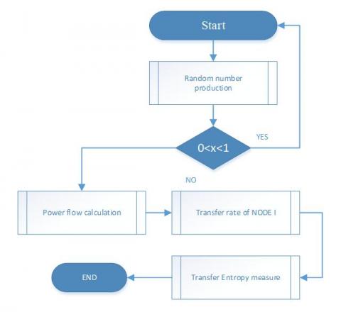
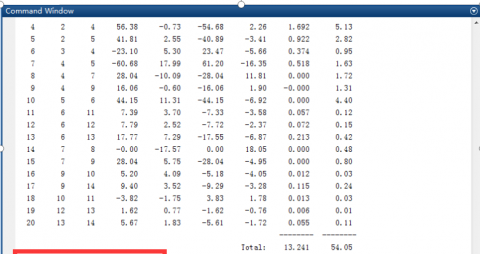
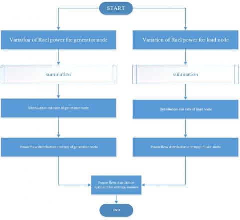
In order to verify the efficiency of mixed entropy measure on IEEE14 network, the different set of experiments are carried out in the MATPOWER toolbox of the MATLAB platform. Moreover the flow charts of power flow transfer entropy and power flow distribution entropy are shown in Figure 2 and Figure 4. Moreover, the experiment results of two entropy methods under MATPOWER toolbox are shown in Figure 3 and Figure 5.

2.jpg

Figure 2. Flow chart of power flow transfer entropy

Compared with the Figure 3 and Figure 5, we can draw the conclusion that the permutation of transfer entropy and distribution entropy are shown in table 8-10. and the sequence of distribution entropy is shown in fig.6.which means that the node 2 is the vulnerabilities in the whole network. The first set is based on IEEE 14 BUS test system. For a comparison between the mixed entropy method and power flow entropy method (or risk entropy method), the different scheduling order are shown in Fig.6 and Fig.7.As can be seen from the Fig.6(mixed entropy method), the node 3,4,5 have the same risk entropy. However, we can only draw the conclusion that the node 2 is the vulnerabilities in the whole network.

3.png

Figure 3. Experiment results of transfer entropy under MATPWOER

4.jpg

Figure 4. Flow chart of power flow of distribution entropy

5.png

Figure 5. Experiment results of distribution entropy under MATPWOER

Table 8. Transfer entropy

number	test1	test2	test3	test4	test5	average
node2	1.298603	1.298620	1.298616	1.298626	1.298620	1.30
node3	1.929835	1.929849	1.929832	1.929824	1.929825	1.93
node4	2.112372	2.112372	2.112372	2.112372	2.112372	2.11
node5	1.828546	1.828548	1.828549	1.828547	1.828549	1.83
node6	2.633288	2.633288	2.633282	2.633289	2.633287	2.63
node9	2.739682	2.739690	2.739687	2.739690	2.739692	2.74
node10	2.683222	2.683221	2.683219	2.683225	2.683216	2.68
node11	2.532113	2.532119	2.532114	2.532116	2.532116	2.53
node12	2.742392	2.742389	2.742391	2.742390	2.742389	2.74
node13	2.716629	2.716629	2.716629	2.716629	2.716629	2.72
node14	2.698687	2.698684	2.698684	2.698688	2.698687	2.70

Table 9. Distribution entropy

Number	test1	test2	test3	test4	test5	average
node2	-0.09355856	-0.08894123	-0.07713753	-0.1428928	-0.1347842	-0.11
node3	-0.6137061	-0.6127401	-0.6151092	-0.6107501	-0.6131079	-0.61
node4	-0.7826699	-0.7856685	-0.7851088	-0.7717788	-0.7743651	-0.78
node5	-0.7570722	-0.7396852	-0.7577844	-0.7399870	-0.7579246	-0.75
node6	-1.335513	-1.339591	-1.340334	-1.331429	-1.333509	-1.34
node9	-1.432500	-1.433163	-1.430637	-1.427934	-1.431422	-1.43
node10	-1.365670	-1.350894	-1.350821	-1.362479	-1.354593	-1.36
node11	-1.285974	-1.295250	-1.287376	-1.291148	-1.291902	-1.29
node12	-1.444787	-1.446974	-1.448250	-1.449639	-1.451017	-1.45
node13	-1.426913	-1.423656	-1.421644	-1.422398	-1.426396	-1.42
node14	-1.384793	-1.392451	-1.390621	-1.388106	-1.388971	-1.39

Table 10. Measure of distribution entropy

Number	2	3	4	5	6	9	10	11	12	13	14
Measure	-0.14*	-1.18	-1.65	-1.37	-3.52	-3.92	-3.64	-3.26	-3.97	-3.86	-3.75

Where * is the maximum value

6.png

Figure 6. Sequence of distribution entropy

7.png

Figure 7. Sequence of risk entropy

4. Conclusion

In this paper, the mixed entropy measure method is proposed to analyze the fragility of the fault of IEEE14 nodes. Compared with the power flow entropy method or the risk entropy method, the proposed method has the advantage that the sequence of distribution entropy can be quantized with the number of distribution entropy. On the other hand, the proposed method can achieve better solutions for the same computational effort. Further research work includes that a high performance method for the power network vulnerability analysis with large nodes.

Acknowledgments

This paper is supported by Natural Science Foundation of Fujian Province under grant (grant number 2016H6019, 2016J01267), in part by Scientific and Technological Projects of Fuzhou City (grant number 2016-G-53), in part by scientific research project of Xiamen City (grant number 3502Z20189033), in part by the Scientific Research Items of MJU [grant number MJY18003]

References

Ardakani A. J., Bouffard F. (2013). Identification of umbrella constraints in DC-based security constrained optimal power flow. IEEE Trans. Power Syst, Vol. 28, No. 4, pp. 3924–3934. http://doi.org/10.1109/TPWRS.2013.2271980

Barocio E., Regalado J., Cuevas E. (2017). Modified bio-inspired optimization algorithm with a centroid decision making approach for solving a mufti-objective optimal power flow problem. IET Generation Transmission & Distribution, Vol. 11, No. 4, pp. 1012-1022. http://doi.org/10.1049/iet-gtd.2016.1135

Bucha B., Janák J. (2014). A MATLAB-based graphical user interface program for computing functionals of the geopotential up to ultra-high degrees and orders. Pergamon Press, Inc. Vol. 56, pp. 186-196. http://doi.org/10.1016/j.cageo.2013.03.012

Capitanescu F. (2011). Contingency filtering techniques for preventive security-constrained optimal power flow. Elect. Power Syst. Res, Vol. 81, No. 8, pp. 1731-1741. http://doi.org/10.1109/TPWRS.2007.907528

Capitanescu F., Wehenkel L. (2012). Sensitivity-based approaches for handling discrete variables in optimal power flow computations. IEEE Trans. Power Syst, Vol. 25, No. 4, pp. 1780–1789. http://doi.org/10.1109/TPWRS.2010.2044426

Carvalho L. D. M., Silva A. M. L. D., Miranda V. (2018). Security-constrained optimal power flow via cross-entropy method. IEEE Transactions on Power Systems, No. 99, pp. 1-1. http://doi.org/10.1109/TPWRS.2018.2847766

Christopher B., Rua M. (2014). Maximum entropy estimates for risk-neutral probability measures with non-strictly-convex data. Journal of Optimization Theory and Applications, Vol. 161, No. 1, pp. 285-307. http://doi.org/ 10.1007/s10957-013-0349-x

Fang R., Shang R., Wang Y. (2017). Identification of vulnerable lines in power grids with wind power integration based on a weighted entropy analysis method. International Journal of Hydrogen Energy, Vol. 42, No. 31. http://doi.org/10.1016/j.ijhydene.2017.06.039

Green M., Pierre P. D., Derby K. (2003). Ground plane insulation failure in the first TPC superconducting coil. IEEE Transactions on Magnetics, Vol. 17, No. 5, pp. 1855-1859. http://doi.org/10.1109/tmag.1981.1061311

Iacoboaiea O. C., Sayrac B., Jemaa S. B. (2016). On mobility parameter configurations that can lead to chained handovers. IEEE Transactions on Communications, Vol. 64, No. 12, pp. 5136-5148. http://doi.org/10.1109/TCOMM.2016.2615613

Kazemdehdashti A., Mohammadi M., Seifi A. R. (2018). The generalized cross-entropy method in probabilistic optimal power flow. IEEE Transactions on Power Systems, No. 99, pp. 1-1. http://doi.org/10.1109/TPWRS.2018.2816118

Marano-Marcolini A., Capitanescu F., Martinez-Ramos J., Wehenkel L. (2012). Exploiting the use of DC SCOPF approximation to improve iterative AC SCOPF algorithms. IEEE Trans. Power Syst, Vol. 27, No. 3, pp. 1459–1466. http://doi.org/10.1109/tpwrs.2012.2186469

Momoh J. A. (2009). Electric Power System Applications of Optimization. Boca Raton, FL, USA: CRC Press.

Monticelli A. J., Pereira M. V. P., Granville S. (1987). Security-constrained optimal power flow with post-contingency corrective rescheduling. IEEE Trans. Power Syst, Vol. 2, No. 1, pp. 175–182. http://doi.org/10.1109/TPWRS.1987.4335095

Phan D., Kalagnanam J. (2012). Some efficient optimization methods for solving the security-constrained optimal power flow problem. IEEE Trans. Power Syst, Vol. 29, No. 2, pp. 836-872. http://doi.org/10.1109/TPWRS.2013.2283175

Platbrood L., Capitanescu F., Merckx C., Crisciu H., Wehenkel L. (2014). A generic approach for solving nonlinear-discrete security-constrained optimal power flow problems in large-scale systems. IEEE Trans. Power Syst, Vol. 29, No. 3, pp. 1194–1203. http://doi.org/10.1109/TPWRS.2013.2289990

Shahidehpour M., Yamin H., Li Z. (2002). Market operations in Electric Power Systems: Forecasting, Scheduling, and Risk Management. Hoboken, NJ, USA: Wiley-IEEE Press.

Stott B., Alsac O., Monticelli A. J. (1987). Security analysis and optimization. Proc. IEEE, Vol. 75, No. 12, pp. 1623-1644. http://doi.org/10.1109/PROC.1987.13931

Thomasian A., Blaum M. (2006). Mirrored disk organization reliability analysis. IEEE Transactions on Computers, Vol. 55, No. 12, pp. 1640-1644. http://doi.org/10.1109/tc.2006.201

Wang Q., McCalley J. D., Tongxin Z., Litvinov E. (2013). A computational strategy to solve preventive risk-based security constrained OPF. IEEE Trans. Power Syst, Vol. 28, No. 2, pp. 1666-1675. http://doi.org/10.1109/tpwrs.2012.2219080

Wang W. Q., Wang D., Singh V. P. (2018). Optimization of rainfall networks using information entropy and temporal variability analysis. Journal of Hydrology, No. 559. http://doi.org/10.1016/j.jhydrol.2018.02.010

Wang Y., Shahidehpour M., Lai L. L. (2018). Resilience-constrained hourly unit commitment in electricity grids. IEEE Transactions on Power Systems, No. 99, pp. 1-1. http://doi.org/10.1109/TPWRS.2018.2817929

Wood A. J., Wollenberg B. F., Sheble G. B. (2014). Power Generation, Operation, and Control. Hoboken. NJ, USA: Wiley.

Zhu J. (2009). Optimisation of Power System Operation. Hoboken, NJ, +USA: Wiley-IEEE Press. http://doi.org/10.3176/oil.2013.2S.01

IJHT
MMEP
ACSM
EJEE
ISI
I2M
JESA
RCMA
RIA
TS
IJSDP
IJSSE
IJDNE
JNMES
IJES
EESRJ
RCES
AMA_A
AMA_B
AMA_C
AMA_D
MMC_A
MMC_B
MMC_C
MMC_D

Username
Password
Remember me

Search form

Reliability analysis and matpower simulation of IEEE14 node based on mixed entropy measure