Imene Djelamda* | Mohamed Seif Eddine Boulkenafet | Redouane Bouaroua
© 2021 IIETA. This article is published by IIETA and is licensed under the CC BY 4.0 license (http://creativecommons.org/licenses/by/4.0/).
OPEN ACCESS
This work presents a field oriented control (FOC) strategy (Fuzzy Logic (FL)) associated with PI controller applied to the control system of an permanent magnet synchronous motor (PMSM) powered by an inverter dedicated to electric vehicles, the major challenge of our research work is a control law for a permanent magnet synchronous motor more efficient in terms of rejection of disturbances; stability and robustness with respect to parametric uncertainties, A comparison of the performance of the proposed FOC with the FOC with the fuzzy-PI will be presented. The overall development scheme is summarized and an example illustrates features of the control approach performed on a 0.5 kW PMSM drive. The torque and the speed will be judged and compared for the two orders offered. As results, the behavior of the FOC based on fuzzy-PI controller is more efficient compared to the conventional vector control.
electric vehicle, permanent magnet synchronous motor (PMSM), field-oriented control (FOC), Fuzzy-PI controller
In electric vehicles based on permanent magnet synchronous motor, in order to avoid mechanical vibrations and speed variations, the resulting torque must be as constant as possible [1].
In order to achieve high efficiency of the entire drive, each part must be designed in relation to all other components so that total losses are truly minimized. A key component in any VE application is the electrical machine; naturally an additional limitation in this optimization procedure is the cost which makes the electrical machine design step even more complicated. Today, permanent magnet machines are the most common types [2, 3], although switched reluctance (due to their low cost and potential for operation in a wide power range).
Permanent magnet machines are due to their high efficiency power density and inertia torque a common choice in EV concepts. In an EV application the electric machine must operate at varying loads and speeds, which requires careful selection of motor parameters by the machine designer to minimize losses permanent magnet machines depend on the waveform of supply voltage, divided into brushless DC machines with trapezoidal voltage waveforms and permanent magnet synchronous machines with sine waveforms, both types are found in VE [4, 5].
Today, permanent magnet synchronous motors are recommended in the industrial world. This is because they are reliable, have a rotational speed proportional to the power supply frequency, and they are less bulky than DC motors due to the elimination of the excitation source. Thus, their construction is simpler since it does not belong to a mechanical collector which leads to major drawbacks such as power limitation, brush wear and rotor losses [6, 7]. Therefore, this in-creases their service life and avoids permanent maintenance Control without speed and position sensors has become an area of intensive research and development [8, 9].
The main goal of fuzzy logic being to achieve a simple adaptive and efficient control [10].
This controller offers the possibility of obtaining the reproduction of the dynamics of a complex nonlinear system only with the inputs outputs.[11]
The researchers want to avoid the problems encountered in regulation systems [12, 13], caused by the imperfections inherent in the rotational motion sensors used. Incorporating these into systems can increase their complexity and size. It can also degrade the performance of the regulation. For these reasons, the removal of these sensors is essential [14, 15].
In 1971, BLASCKE proposed a field-oriented control theory (FOC) which makes it possible to assimilate the behavior of the PMSM to a DC machine with separate excitation, the control law corresponding to this dynamic mode of action are gathered under the name vector control, the main objective of which is therefore to control the torque in an optimal way according to a chosen criterion [16].
On the other hand, several modern strategies applied to permanent magnet synchronous machines such as control by fuzzy logic [17].
The main goal of fuzzy logic being to achieve a simple adaptive and efficient control [10].
This controller offers the possibility of obtaining the reproduction of the dynamics of a complex nonlinear system only with the inputs outputs [11].
This article describes the fuzzy logic and the classical PI regulator that will be introduced in the vector control of the permanent magnet synchronous machine. The general principle and basic theory of FOC control will be presented first. Then the artificial intelligence technique is applied to the FOC control.
Mathematical model of the PMSM system can be expressed by such equations in the rotating reference frame (d-q reference frame). Accordingly, the rotor reference plane of the PMSM equivalent circuit can be shown as in Figure 1.
Figure 1. PMSM dq-axis dynamic equivalent circuit [17]
Stator dq equations can be written in the rotor reference plane of PMSM using Figure 1 as:
$V_{d}=R_{s} i_{d}+L_{d} \frac{d i_{d}}{d t}-\omega_{e} \lambda_{q}$ (1)
$V_{q}=R_{s} i_{q}+L_{q} \frac{d i_{q}}{d t}+\omega \lambda_{e d}$ (2)
where Vd and Vq are dq-axis voltages, id and iq are dq axis currents, λd and λq are dq-axis fluxes and ωe is the electrical rotor speed. The fluxes are described in Eqns. (3) and (4) [4].
$\lambda_{d}=L_{d} i_{d}+\lambda_{m}$ (3)
$\lambda_{q}=L_{q} i_{q}$ (4)
The expression of λm represents mutual magnetic flux caused by the permanent magnet:
$T_{e m}=\frac{3}{2} P\left(\lambda_{m} i_{g}\right)\left(L_{d}-L_{q}\right)\left(i_{d} \cdot i_{q}\right)$ (5)
For constant flux operation, the electromagnetic torque is:
$T_{e m}=\frac{3}{2} P\left(\lambda_{m} i_{q}\right)$ (6)
P is the number of pairs of poles.
$T_{e m}=T_{L}+B . \omega_{r}+J . d \omega_{r} d t$ (7)
$\omega_{r}=\int\left(\frac{T_{e m}-T_{r}-B \omega_{r}}{J}\right) d t$ (8)
where, ωr is the mechanical speed, J is the inertia moment of the motor and Tr is the load torque.
The parametric identification of an electric machine is a first phase of its modeling. The importance of electric machines, in particular in variable speed systems, is such that the reliability of any study is largely dependent on the precision of the models on the one hand, and on the other hand on the experimental methods for the identification of the parameters contained therein in the model [8-18].
Among the parametric identification methods, we can cite those based on the classical tests of synchronous machines highly recommended by the International Electrotechnical Commission (CEl). Scale attack index trials could also reveal parameters of synchronous machines [8].
3.1 Exploiting the nameplate of PMSM
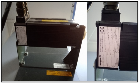
Table 1 shows the various parameters taken from the nameplate of the permanent magnet synchronous motor used in this work. Figure 2 depicts the PMSM machine.
Table 1. PMSM nameplate data
|
Nmax |
Tn |
In |
2P |
BEMF |
|
3000 rpm |
4.9 N.m |
5.56 A |
6 |
62.5 V/kRPM |
Figure 2. PMSM machine
3.2 The tests to identify the parameters of the PMSM
One of the possible methods to adjust the PI controller gains is to calculate them from the motor parameters. The gains of the current controllers in the time domain are calculated from the electrical parameters of the motor [8].
The necessary electrical parameters are shown in Table 2.
Table 2. Electrical Parameters
|
Parameter |
Dimension |
Designation |
|
Rs |
Ω |
Stator resistance |
|
Ld |
H |
Direct axis inductance |
|
Lq |
H |
Quadrature axis inductance |
|
Ke |
V.s/ rad |
Electric constant |
|
P |
/ |
Number of pole pairs |
Table 3. Mechanical Parameter
|
Parameter |
Dimension |
Designation |
|
J |
Kg.m2 |
Moment of inertia |
|
f |
N.m.s/rad |
Coefficient of viscous friction |
The speed regulator gains in the time domain are calculated from the mechanical parameters (motor / load) in Table 3.
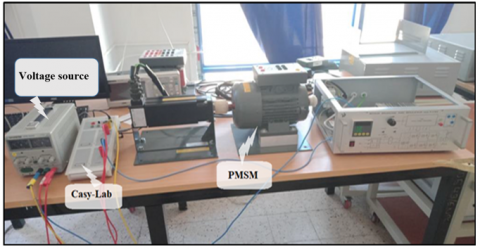
A test bench was prepared to carry out the various tests to identify the electrical and mechanical parameters represented in Figure 3.
Figure 3. Identification test bench
3.2.1 Identification of the number of pole pairs
Usually, the number of motor pole pairs is listed on the motor nameplate. If there is no information regarding the number of pole pairs, it can be determined by the tests below:
The motor is rotated by an external drive motor at a constant speed N = 1500 rpm (Figure 4).
The voltage curve generated by the permanent magnet synchronous machine is saved using the Cassy-Lab.
The frequency of the voltage generated by the permanent magnet synchronous machine is measured
The engine speed is measured by a hand-held tachometer.
We calculate the number of pairs of poles.
Figure 4. Voltage curve obtained for N = 1500 rpm
$P=60 \mathrm{f} / n$ (9)
f is the frequency with:
$f=1 / T$ (10)
After calculating we find that P = 3.
3.2.2 Identification of stator resistance
If the nameplate does not indicate any reference resistance, the following Ohmmeter (or digital multimeter) method can be used [12]:
We flick the measuring instrument between two phases and we will find the resistance value from the following Two relations:
If the stator is connected in star:
$R s=R / 2$ (11)
If the stator is connected in delta:
$R s=3 . R / 2$ (12)
3.2.3 Identification of synchronous inductors
Tests for the identification of synchronous inductance Ld.
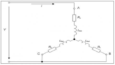
The rotor is aligned along the d axis, phase A is connected to the positive potential, and the other two phases (C and B) to ground according to Figure 5 [8].
We block the rotor shaft.
A voltage step is applied; phase A is grounded and the other two phases connected to the positive potential (The usual level of the current is about 10% of the nominal current of the phase).
The current measurements are taken by Cassy-Lab.
We calculate the inductance Ld from the time constant of the current response.
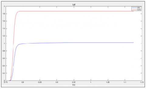
Figure 6 represents the voltage step and the current response as a function of time.
Figure 5. Inductance measurement setup Ld [12]
Figure 6. Voltage and current curve as a function of time for the test of Ld
$L_{d, q}=\tau . R_{s} / 2$ (13)
Test for the identification of synchronous inductance Lq.
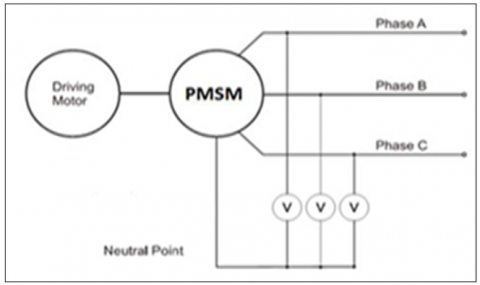
3.2.4 Identification of the constant Ke Back_EMF
The constant Ke is obtained by measuring the phase-to-neutral voltage Vpk of the motor while it is being driven by an external drive motor at a constant speed. The constant Ke is defined as the BEMF voltage in each of the phases per unit of rotation speed [18].
We run the PMSM by an external drive motor at a constant speed, in our case n = 1207 rpm.
We measure the compound voltage between two phases.
We calculate the BEMF constant by the following equation:
$K_{e}=V_{p k} / \omega_{e l}=\left(V_{p k-p k} \cdot T_{e l}\right) / 2 . \Pi$ (14)
After carrying out the diagram (Figure 7), we obtained the voltage curve of phase A and B by Cassy Lab (Figure 8):
Figure 7. Three-phase voltage measurement diagram of the constant Ke [12]
Figure 8. Voltage curve of phase A and B as a function of time
Peak to peak line voltage: $V_{p k-p k}=218.4 \mathrm{~V}$.
The period: $T=16.2 \mathrm{~ms}$.
A numerical map on Eq. (13) and we find that:
$K e=0.5631 \mathrm{~V} . \mathrm{s} / \mathrm{rad} \Rightarrow \mathrm{Ke}=58.96 \mathrm{~V} / \mathrm{kRPM}$.
3.2.5 Identification of mechanical parameters
No-load test of PMSM
In this test we supplied the motor with a voltage = 300 V, the motor rotates at a speed equal to 3000 rpm, at this point, we noted the no-load current, the active power consumed no-load, using the two-wattmeter method see the Table 4.
We calculate the mechanical losses using the following relation:
$P_{0}=P_{\text {mec }}+P_{\text {fer }}=2 P_{\text {mec }}$ (15)
Table 4. Power measured by the two-wattmeter
|
V0(V) |
I0(A) |
W1(W) |
W2(W) |
P0(W) |
|
300 |
1~1.4 |
65 |
70 |
135 |
Method used to determine the mechanical parameters, consists in controlling the MSAP assembly coupled to the induction machine using a speed variator.
The machine starts up to reach the maximum speed of 3000 rpm. Then, the power is cut off at this speed and the machine decelerates via mechanical losses.
We record the speed deceleration and we get the mechanical speed decrease curve in this experiment [19] (Figure 9):
Figure 9. Voltage curve versus time of the deceleration test
We calculate the moment of inertia and the coefficient of friction from the following equations:
$P_{m e c}=J. \Omega_{\max } \cdot d \Omega / d t$ (16)
$\tau_{m}=J / f$ (17)
The characteristics of the MSAP studied are shown in the Table 5.
Table 5. PMSM parameters
|
Parameter |
Symbol |
Value |
|
Nominal power |
$P_{n}$ |
513.12 W |
|
Nominal torque |
$T_{n}$ |
4.9 N.m |
|
Nominal speed |
$N_{n}$ |
1000 tr/min |
|
Maximum speed |
$N_{\max }$ |
3000 tr/min |
|
Stator resistance |
$R_{s}$ |
2.2 $\Omega$ |
|
Direct axis inductance |
$L_{d}$ |
12.65 mH |
|
Quadrature axis inductance |
$L_{q}$ |
12.65 mH |
|
Magnets flux |
$\Phi_{s f}$ |
0.27 Wb |
|
Number of poles |
$2 p$ |
6 pôles |
|
Moment of inertia |
J |
0.000715 Kg.m2 |
|
Coefficient of friction |
f |
0.001489 N.m.s/rad |
|
Supply voltage |
$V_{n}$ |
124 V |
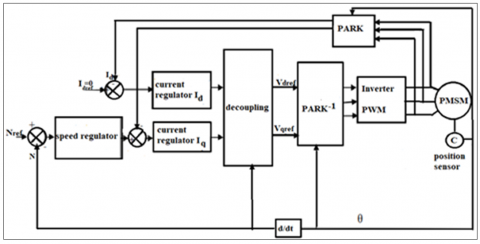
The principle of vector control is identical to that of controlling a DC machine with separate excitation, it consists of regulating the flow by one component of the current and the torque by the other component (Figure 10).
The purpose of this command is to orient the rotor flux along the d axis, this strategy is to keep the d axis constantly aligned with the flux vector of the magnet [3].
The reference for the current id is kept at zero, the reference for the current iq is de-terminated by means of a speed Integral-Proportional (PI) corrector. This regulator has the advantage of not introducing zero in the closed loop transfer function while ensuring zero static error. In this command, we will use the non-linear type decoupling in order to close the regulation loop of Park currents through Proportional-Integral (PI) regulators [5].
$i d=0 \Rightarrow \lambda d=\lambda_{s f}$ (18)
$T_{e m}=K \cdot i_{q} \rightarrow$ Tem $=3 . P. \lambda_{s f} \cdot i_{q} / 2$ (19)
The model of the machine in Park's frame becomes:
$V d=-\omega_{r} L_{q} i_{q}$ (20)
$V_{q}=R_{s} i_{q}+L_{q}. d i q / d t+\omega_{r} \lambda_{s f}$ (21)
Figure 10. Diagram of the vector control [9]
The inputs of the fuzzy controller FLC are: the error and the derivative of the error of, the outputs are: the normalized value of the proportional action kp and the normalized value of the integral action ki (Figure 11).
Figure 11. Membership function form
The fuzzy subsets of the input variables are defined as shown in Table 6. knowing that ‘e’ is the speed error and ‘de’ is the derivation of speed error
Table 6. Seven class command rules table
|
de e |
NG |
NM |
NP |
Z |
PP |
PM |
PG |
|
NG |
NP |
NP |
NP |
NP |
NM |
NG |
Z |
|
NM |
NG |
NG |
NG |
NM |
NP |
Z |
PP |
|
NP |
NG |
NG |
NM |
NP |
Z |
PP |
PM |
|
Z |
NP |
NM |
NG |
Z |
PP |
PM |
PG |
|
PP |
NM |
NP |
Z |
PP |
PM |
PG |
PG |
|
PM |
NP |
Z |
PP |
PM |
PG |
PG |
PG |
|
PG |
Z |
PP |
PM |
PG |
PG |
PG |
PG |
6.1. Results and discussion
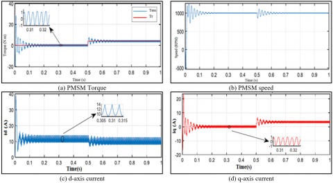
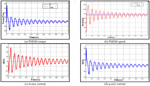
This test is carried out with a speed step Nref= 750 rpm with application of a load $\operatorname{Tr}=4 N \cdot m$ (0.5 s), supplied by a voltage inverter.
We notice that the speed takes very important peaks at the beginning (Figure 12b) then stabilizes at the speed of synchronism.
The speed quickly reaches steady state this being due to the low inertia of the PMSM. This imposes a short response time of 0.2 s. In steady state the speed remains constant and equal to the synchronism speed 1000 rpm, until the application of Cr = 4 N.m at t = 0.5 s, then we see that the speed takes peaks but always stabilizes at the synchronous speed despite the application of the load.
According to (Figure 12a) there is a very high starting torque 37 N.m, the latter stabilizes in the vicinity of zero; at 0.5 S the electromagnetic torque responds quickly to the load demand and stabilizes at the same value of the resistive torque 4 N.m.
Figure 12. Performance of PMSM
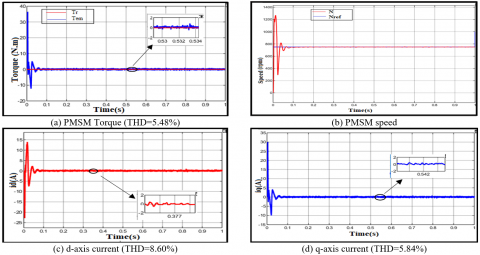
Figure 13. Performance of FOC applied to PMSM
Figure 14. Performance of Fuzzy-PI controller associate with FOC applied to the PMSM
When applying the FOC (Figure 13); the starting torque is high, the latter stabilizes around zero since there is no load, the speed following the reference with a response time t = 0.07 s, overshoot and static error non zero.
From the response of performance of Fuzzy-PI controller associate with FOC applied to PMSM (Figure 14) the speed follows the reference perfectly with a very short response time t = 0.02 s, overshoot and zero static error.
The starting torque is high, it stabilizes around zero since there is no load.
When applying some faults short circuit (Figure 15) and (Figure 16), open circuit (Figure 17) and (Figure 18), moment of inertia defect (Figure 19) and (Figure 20) we notice the robustness of the fuzzy-PI controller associated with the FOC compared to the FOC only.
Figure 15. Performance of FOC applied to PMSM (short circuit 5%)
Figure 16. Performance of Fuzzy-PI controller associate with FOC applied to PMSM (short circuit 5%)
Figure 17. Performance of FOC applied to PMSM (open circuit 5%)
Figure 18. Performance of Fuzzy-PI controller Associate with FOC applied to PMSM (open circuit 5%)
Figure 19. Performance of FOC applied to PMSM (J=10%J)
Figure 20. Performance of Fuzzy-PI controller associate with FOC applied to PMSM (J=10%J)
In this article we have highlighted the improvement brought by the fuzzy-PI associated with vector control on the performance of the permanent magnet synchronous motor compared to the vector control only.
The simulation results showed: a remarkable behavior of the adaptive Flou-PI controller in regulation and in tracking, a disturbance rejection much better than for the other regulators, very good performances with regard to robustness. Thus, the use of such a hybrid solution (PI adjusted by an FLC) makes it possible to rationally exploit the advantages of classical and fuzzy PI regulators and to overcome their drawbacks.
[1] John, S., Rasheed, A.I., Reddy, V.K. (2013). ASIC implementation of fuzzy-PID controller for aircraft roll control. In 2013 International Conference on Circuits, Controls and Communications (CCUBE), Bengaluru, India, pp. 1-6. https://doi.org/10.1109/CCUBE.2013.6718551
[2] Savelyev, D.O., Gudim, A.S. (2018). Software fuzzy logic compensator of nonlinear elements of automatic control system. In 2018 International Multi-Conference on Industrial Engineering and Modern Technologies (FarEastCon), Vladivostok, pp. 1-4. https://doi.org/10.1109/FarEastCon.2018.8602829
[3] Hosseyni, A., Trabelsi, R., Mimouni, M.F., Iqbal, A. (2014). Vector controlled five-phase permanent magnet synchronous motor drive. In 2014 IEEE 23rd International Symposium on Industrial Electronics (ISIE), Istanbul, Turkey, pp. 2122-2127. https://doi.org/10.1109/ISIE.2014.6864945
[4] Chan, C.C. (2002). The state of the art of electric and hybrid vehicles. Proceedings of the IEEE, 90(2): 247-275. https://doi.org/10.1109/5.989873
[5] F. Ben Ammar, High performance variable speed drive for high power asynchronous machines, Thesis of the National Polytechnic Institute of Toulouse, N ° 708, 1993
[6] Pillay, P., Krishnan, R. (1987). Modeling of permanent magnet motor drives. In IECON'87: Motor Control and Power Electronics, 854: 289-293. https://doi.org/10.1117/12.942973
[7] Sebba, M., Chaker, A., Meslem, Y., Hassaine, S. (2007). Commande en vitesse du moteur synchrone à aimants permanents dotée d’un observateur d’état de Luenberger. In 4th International Conference on Computer Integrated Manufacturing.
[8] Abdessemed, R. (2011). Électrotechnique-Modélisation et Simulation des Machines. Ellipses.
[9] Chebre, M., Zerikat, M., Bendaha, Y. (2007). Adaptation des paramètres d’un contrôleur PI par un FLC appliqué à un moteur asynchrone. In 4th International Conference on Computer Integrated Manufacturing CIP, pp. 3-4.
[10] Uysal, A., Gokay, S., Soylu, E., Soylu, T., Çaşka, S. (2019). Fuzzy proportional-integral speed control of switched reluctance motor with MATLAB/Simulink and programmable logic controller communication. Measurement and Control, 52(7-8): 1137-1144. https://doi.org/10.1177%2F0020294019858188
[11] Macriga, A., Kruthiga, K., Anusudha, S. (2017). Artificial voice synthesizer using fuzzy logics. In 2017 2nd International Conference on Computing and Communications Technologies (ICCCT), Chennai, India, pp. 388-392. https://doi.org/10.1109/ICCCT2.2017.7972313
[12] Bobek, V. (2013). PMSM electrical parameters measurement. Freescale Semiconductor, 7(8): 13.
[13] Grellet, G., Clerc, G. (1997). Actionneur Electriques. Principes, Modèles, Commande. Eyrolles.
[14] Mehedi, F., Nezli, L., Mahmoudi, M.O., Taleb, R., Boudana, D. (2019). Fuzzy logic based vector control of multi-phase permanent magnet synchronous motors. Journal of Renewable Energies, 22(1): 161-170.
[15] Dursun, M., Boz, A.F. (2015). The analysis of different techniques for speed control of permanent magnet synchronous motor. Tehnički vjesnik, 22(4): 947-952. https://doi.org/10.17559/TV-20140912141639
[16] Maamoun, A., Alsayed, Y.M., Shaltout, A. (2013). Fuzzy logic based speed controller for permanent-magnet synchronous motor drive. In 2013 IEEE International Conference on Mechatronics and Automation, Takamatsu, Japan, pp. 1518-1522. https://doi.org/10.1109/ICMA.2013.6618139
[17] Nabti, K. (2010). Stratégie de commande et techniques intelligentes appliquées aux machines de type synchrone. Thèse de Doctorat, Université Mentouri Constantine.
[18] Permanent magnet synchronous motor with sinusoidal flux distribution. Math Works, 2021. https://www.mathworks.com/help/physmod/sps/ref/pmsm.html.
[19] Nyoumea, G.P. (2018). Modèles d'identification et de commande d'un aérogénérateur à machine synchrone à aimants permanents. Doctoral dissertation.