Horch Mohamed* | Boumédiène Abdelmadjid | Baghli Lotfi
© 2020 IIETA. This article is published by IIETA and is licensed under the CC BY 4.0 license (http://creativecommons.org/licenses/by/4.0/).
OPEN ACCESS
This paper aims to propose an improved Direct Torque Control (DTC) strategy with Space Vector Modulation (SVM) for induction machines (IM). The performance enhancement is operated by using the nonlinear backstepping strategy. This approach is proposed to ensure a robust control against different uncertainties and external disturbances and to reduce torque and flux ripples. The backstepping controller uses the stator resistance of the machine for estimation of the stator flux. The variations of the stator resistance due to the changes in temperature or frequency make the operation of this control difficult at low speeds. A new method for the estimation of stator resistance changes during machine operation is proposed. It is based on a Super Twisting strategy. The design of the proposed DTC strategy law is developed theoretically and realized through numerical simulations. Different operating conditions are applied to check the ability and robustness of the proposed control strategy, such as steady state, speed reversal maneuver, low-speed operation, parameters variation and load application. Results clearly show improvement in DTC at low speeds.
induction machine, nonlinear control, backstepping, direct torque control, space vector modulation stator resistance compensator, super twisting strategy
In the studies of variable speed electric drives, it appears that the induction machine is the most electromechanical robust of alternative machines in terms of parameters robustness, construction and maintenance [1].
However, the development of control strategies to control the speed of induction machine is necessary, because this machine is characterized by a multivariable and nonlinear mathematical model, with a strong coupling between the control factors. Considerable research effort is carried to find control strategies with good performances and suitable for induction machines [2].
In the recent decades, several control strategies were developed and improved, among these strategies, the Direct Torque Control, which was proposed in 1985 by Takahashi et al. [2]. The DTC is a well-known strategy in electrical engineering, lately it is increasingly used in industrial applications, compared to other types of control and more particularly the vector control, its main advantages is that it allows a very fast torque response and has a low machine parameters dependency.
The DTC exploits the possibility of imposing a torque and a stator flux to the IM in a decoupled manner, when they are powered by a voltage fed inverter without the use of a feedback loop for the current control, achieving a performance similar to that of field oriented control. It consists of controlling the stator flux and the electromagnetic torque magnitudes with nonlinear hysteresis controllers. The output of these controllers determines the optimum voltage vector to be applied at each switching instant [3, 4].
However, two major disadvantages arise. On one hand, the determination of the switching states is based on information on the evolution trends of the flux and the torque resulting from the nonlinear hysteresis controllers, and on the other hand, since the duration of the commutations is variable, this leads to rise oscillations of torque and stator flux [5].
The use of these nonlinear hysteresis controllers creates oscillations on the variables to be controlled [6]. In this case, it is necessary to apply a constant modulation frequency using the space vector modulation (SVM). A hybrid method, combining conventional DTC control with nonlinear control design based on backstepping controllers is used. The hysteresis blocks are replaced to reduce torque and flux ripples and ensure a robust control against different uncertainties and external disturbances. Its main feature is the removal of the hysteresis controllers and switching table, eliminating the problems they induce [6].
In the relatively high-speed operating conditions of the IM, there is no influence of the resistive term on the performance of the DTC. This is no longer true for very low speeds, because of the incorrect value of the stator resistance, due to bad identification or temperature variations [7-9]. This certainly impacts the estimation of the stator flux and the electromagnetic torque magnitudes, and thus leading to serious malfunctions in the choice of the voltage vector to be applied to the inverter. The contribution of this paper is the development of a new stator resistance compensator based on a super-twisting control algorithm to estimate the variation of the stator resistance of the machine during operation.
The paper parts are structured as follows: section 2 shows the mathematical model of the induction machine. In section 3 we applied a DTC technique approach of the torque associated with the backstepping approach, then we have improved the direct torque control using a new stator resistance compensator. Finally, we present conclusions and perspectives.
The mathematical model of the IM is described in the stationary reference frame by the following nonlinear equations [10, 11]:
$\left\{\begin{array}{l}\dot{\mathrm{i}}_{\mathrm{s} \alpha}=\mathrm{a}_{1} \mathrm{i}_{\mathrm{s} \alpha}-\mathrm{p} \omega_{\mathrm{r}} \mathrm{i}_{\mathrm{s} \beta}+\mathrm{a}_{2} \phi_{\mathrm{s} \alpha}+\mathrm{a}_{3} \mathrm{p} \omega_{\mathrm{r}} \phi_{\mathrm{s} \beta}+\mathrm{b} \mathrm{v}_{\mathrm{s} \alpha} \\ \dot{\mathrm{i}}_{\mathrm{s} \beta}=\mathrm{a}_{1} \mathrm{i}_{\mathrm{s} \beta}+\mathrm{p} \omega_{\mathrm{r}} \mathrm{i}_{\mathrm{s} \alpha}+\mathrm{a}_{2} \phi_{\mathrm{s} \beta}-\mathrm{a}_{3} \mathrm{p} \omega_{\mathrm{r}} \phi_{\mathrm{s} \alpha}+\mathrm{b} \mathrm{v}_{\mathrm{s} \beta}\\ \dot{\phi}_{\mathrm{s} \alpha}=\mathrm{v}_{\mathrm{s} \alpha}-\mathrm{R}_{\mathrm{s}} \mathrm{i}_{\mathrm{s} \alpha} \\ \dot{\phi}_{\mathrm{s} \beta}=\mathrm{v}_{\mathrm{s} \beta}-\mathrm{R}_{\mathrm{s}} \mathrm{i}_{\mathrm{s} \beta} \\ \dot{\omega}_{\mathrm{r}}=\mathrm{a}_{3} \mathrm{T}_{\mathrm{em}}-\mathrm{a}_{5} \omega_{\mathrm{r}}-\mathrm{a}_{3} \mathrm{T}_{\mathrm{r}}\end{array}\right.$ (1)
The electromagnetic torque equation is:
$\mathrm{T}_{\mathrm{en}}=\mathrm{a}_{4}\left(\mathrm{i}_{\mathrm{s} \beta} \phi_{\mathrm{s} \alpha}-\mathrm{i}_{\mathrm{s} \alpha} \phi_{\mathrm{s} \beta}\right)$ (2)
With the parameters $a_{1}, a_{2}, a_{3}, a_{4}, a_{5}, \sigma$ and b are defined by:
\[\begin{align} & {{a}_{1}}=-\left( \frac{{{R}_{s}}}{\sigma {{L}_{s}}}+\frac{{{R}_{r}}}{\sigma {{L}_{r}}} \right),\text{ }{{a}_{2}}=b\left( \frac{{{R}_{r}}}{(\sigma {{L}_{s}}{{L}_{r}}} \right),{{a}_{3}}=\frac{1}{J}\text{ },{{a}_{4}}=\frac{3}{2}\text{ }p,\text{ } \\ & {{a}_{5}}=\frac{{{f}_{v}}}{J}\text{ },\text{ }\sigma =1-\frac{L_{m}^{2}}{{{L}_{s}}{{L}_{r}}},\text{ }b=\frac{1}{\sigma {{L}_{s}}} \\ \end{align}\]
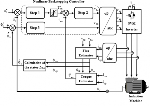
In this section, we applied a DTC technique approach of the torque associated with the backstepping approach to control the stator flux and the torque module of the IM powered by an inverter controlled by the technique SVM. For this method, the hysteresis controllers were replaced by sliding mode controllers, to overcome the problem of the ripple. The Figure 1 illustrates the block diagram for the induction machine control based on the DTC- backstepping approach [12].
3.1 Step 1 (Speed control loop)
In order to design a backstepping control law for speed tracking, the tracking errors are defined as follows:
$\mathrm{e}_{1}=\omega_{\mathrm{r}}^{*}-\omega_{\mathrm{r}}$ (3)
The dynamics of the error is given by:
$\dot{\mathrm{e}}_{1}=\dot{\omega}_{\mathrm{r}}^{*}-\mathrm{a}_{3} \mathrm{T}_{\mathrm{em}}+\mathrm{a}_{5} \omega_{\mathrm{r}}+\mathrm{a}_{3} \mathrm{T}_{\mathrm{r}}$ (4)
In order to elaborate a backstepping control law allowing the speed tracking, one chooses the function of Lyapunov as follows:
$V_{1}=\frac{1}{2}\left(\mathrm{e}_{1}\right)^{2}$ (5)
The Lyapunov function derivative is given by:
$\dot{\mathrm{V}}_{1}=\mathrm{e}_{1}\left(\dot{\omega}_{\mathrm{r}}^{*}-\mathrm{a}_{3} \mathrm{T}_{\mathrm{en}}+\mathrm{a}_{5} \omega_{\mathrm{r}}+\mathrm{a}_{3} \mathrm{T}_{\mathrm{r}}\right)$ (6)
Figure 1. Control scheme based on the DTC-Backstepping approach of IM
In order to have ( $\dot{V}_{1}<0$), the virtual control $T_{e m}^{*}$ that represents the stabilizing function is defined by:
$\mathrm{T}_{\mathrm{em}}^{*}=\frac{1}{\mathrm{a}_{3}}\left(\dot{\omega}_{\mathrm{r}}^{*}+\mathrm{a}_{5} \omega_{\mathrm{r}}+\mathrm{a}_{3} \mathrm{T}_{\mathrm{r}}+\mathrm{K}_{1} \mathrm{e}_{1}\right)$ (7)
where, K1 is a positive constant.
By replacing Eq. (7) in Eq. (4), the dynamic of the error is expressed as:
$\dot{\mathrm{e}}_{1}=-\mathrm{K}_{1} \mathrm{e}_{1}$ (8)
The Lyapunov function becomes:
$\mathrm{V}\left(\mathrm{e}_{1}\right)=\frac{1}{2}\left(\mathrm{e}_{1}\right)^{2}$ (9)
Its derivative is expressed as:
$\dot{\mathrm{V}}\left(\mathrm{e}_{1}\right)=\mathrm{e}_{1} \dot{\mathrm{e}}_{1}=-\mathrm{K}_{1}\left(\mathrm{e}_{1}\right)^{2}$ (10)
So, the error e1 tends to zero and therefore ωr to $\omega_{r}^{*}$.
Since $T_{e m}^{*}$ is not the input control, a second step is necessary, an error variable e2 is chosen to display the input control vsα.
3.2 Step 2 (Torque control loop)
Once the virtual control $T_{e m}^{*}$ is calculated, the error of the torque and its reference is characterized by:
$\mathbf{e}_{2}=T_{\mathrm{em}}^{*}-\mathrm{T}_{\mathrm{em}}$ (11)
The dynamics of this error is given by:
$\dot{\mathrm{e}}_{2}=\dot{\mathrm{T}}_{\mathrm{em}}^{*}-\dot{\mathrm{T}}_{\mathrm{em}}$ (12)
Taking into account the expression (2) and (7), then (12) is rewritten in the following form:
$\begin{array}{l}\dot{\mathrm{e}}_{2}=\frac{1}{\mathrm{a}_{3}}\left(\ddot{\omega}_{\mathrm{r}}^{*}+\mathrm{a}_{5} \dot{\omega}_{\mathrm{r}}+\mathrm{a}_{3} \dot{\mathrm{T}}_{\mathrm{r}}+\mathrm{K}_{1} \dot{\mathrm{e}}_{1}\right) \\ -\mathrm{a}_{4}\left(\dot{\mathrm{i}}_{\mathrm{s \beta}} \phi_{\mathrm{s \alpha}}+\mathrm{i}_{\mathrm{s \beta}} \dot{\phi}_{\mathrm{s} \alpha}-\dot{\mathrm{i}}_{\mathrm{s} \alpha} \phi_{\mathrm{s} \beta}-\mathrm{i}_{\mathrm{s} \alpha} \dot{\phi}_{\mathrm{s\beta}}\right)\end{array}$ (13)
By substituting in the induction machine model (1), we find:
$\begin{align} & {{{\dot{e}}}_{2}}=\frac{1}{{{a}_{3}}}\left( \ddot{\omega }_{r}^{*}+{{a}_{5}}{{{\dot{\omega }}}_{r}}+{{a}_{3}}{{{\dot{T}}}_{r}}+{{K}_{1}}(\dot{\omega }_{r}^{*}-{{{\dot{\omega }}}_{r}}) \right) \\ & -{{a}_{4}}\left( ({{a}_{1}}{{i}_{s\beta }}+p{{\omega }_{r}}{{i}_{s\alpha }}+{{a}_{2}}{{\phi }_{s\beta }}-{{a}_{3}}p{{\omega }_{r}}{{\phi }_{s\alpha }}+b{{v}_{s\beta }}){{\phi }_{s\alpha }} \right.+{{i}_{s\beta }}({{v}_{s\alpha }}-{{R}_{s}}{{i}_{s\alpha }}) \\ & -({{a}_{1}}{{i}_{s\alpha }}-p{{\omega }_{r}}{{i}_{s\beta }}+{{a}_{2}}{{\phi }_{s\alpha }}+{{a}_{3}}p{{\omega }_{r}}{{\phi }_{s\beta }}+b{{v}_{s\alpha }}){{\phi }_{s\beta }}\left. -{{i}_{s\alpha }}({{v}_{s\beta }}-{{R}_{s}}{{i}_{s\beta }}) \right) \\\end{align}$ (14)
We put $\dot{e}_{2}$ in the form:
$\dot{\mathrm{e}}_{2}=\beta_{1}+\beta_{2} \mathrm{v}_{\mathrm{s} \alpha}+\beta_{3} \mathrm{v}_{\mathrm{s} \beta}$ (15)
with:
$\begin{align} & {{\beta }_{1}}=\frac{1}{{{a}_{3}}}\left( \ddot{\omega }_{r}^{*}+{{K}_{1}}\dot{\omega }_{r}^{*}+\left( {{a}_{5}}-{{K}_{1}} \right){{{\dot{\omega }}}_{r}}+{{a}_{3}}{{{\dot{T}}}_{r}} \right) \\ & {{\mathop{{}}_{{}}}_{{}}}-{{a}_{1}}{{a}_{4}}\left( {{i}_{s\beta }}{{\phi }_{s\alpha }}-{{i}_{s\alpha }}{{\phi }_{s\beta }} \right)-{{a}_{4}}p{{\omega }_{r}}\left( {{i}_{s\alpha }}{{\phi }_{s\alpha }}+{{i}_{s\beta }}{{\phi }_{s\beta }} \right)+{{a}_{4}}{{a}_{3}}bp{{\omega }_{r}}\phi _{s}^{2} \\ & {{\beta }_{2}}={{a}_{4}}\left( b{{\phi }_{s\beta }}-{{i}_{s\beta }} \right) \\ & {{\beta }_{3}}={{a}_{4}}\left( {{i}_{s\alpha }}-b{{\phi }_{s\alpha }} \right) \\ \end{align}$
$\phi _{s}^{2}=\phi _{s\alpha }^{2}+\phi _{s\beta }^{2}$
The second function of Lyapunov is chosen such as:
$\mathrm{V}_{2}=\frac{1}{2}\left(\mathrm{e}_{2}\right)^{2}$ (16)
Its derivative is expressed as:
$\dot{\mathrm{V}}_{2}=\mathrm{e}_{2}\left(\beta_{1}+\beta_{2} \mathrm{v}_{\mathrm{s} \alpha}+\beta_{3} \mathrm{v}_{\mathrm{s} \beta}\right)$ (17)
To satisfy the condition ($\dot{v}_{2}<0$), one has to choose vsα and vsβ control inputs as follow:
$\beta_{2} \mathrm{v}_{\mathrm{s} \alpha}+\beta_{3} \mathrm{v}_{\mathrm{s} \beta}=-\beta_{1}-\mathrm{K}_{2} \mathrm{e}_{2}$ (18)
where, K2 is a positive constant.
By replacing Eq. (18) in Eq. (17), the Lyapunov function derivative function of the electromagnetic torque becomes:
$\dot{\mathrm{V}}_{2}=-\mathrm{K}_{2}\left(\mathrm{e}_{2}\right)^{2} \leq 0$ (19)
The derivative of the Lyapunov function (19) is defined as semi negative, so the error e2 tends to zero.
3.3 Step 3 (Flux control loop)
The error of the measured flux and its reference is characterized by:
$\mathrm{e}_{3}=\left(\phi_{\mathrm{s}}^{*}\right)^{2}-\left(\phi_{\mathrm{s}}\right)^{2}$ (20)
The dynamics of e3 is given by:
$\dot{\mathbf{e}}_{3}=2 \dot{\phi}_{\mathrm{s}}^{*}-2\left(\phi_{\mathrm{s} \alpha} \dot{\phi}_{\mathrm{s} \alpha}+\phi_{\mathrm{s} \beta} \dot{\phi}_{\mathrm{s} \beta}\right)$ (21)
Substituting in the model of the machine Eq. (1), we find:
$\dot{\mathrm{e}}_{3}=2 \dot{\phi}_{\mathrm{s}}^{*}-2\left(\phi_{\mathrm{s} \alpha}\left(\mathrm{v}_{\mathrm{s} \alpha}-\mathrm{R}_{\mathrm{s}} \mathrm{i}_{\mathrm{s} \alpha}\right)+\phi_{\mathrm{s} \beta}\left(\mathrm{v}_{\mathrm{s} \beta}-\mathrm{R}_{\mathrm{s}} \mathrm{i}_{\mathrm{s} \beta}\right)\right)$
We put $\dot{e}_{3}$ in the form:
$\dot{\mathrm{e}}_{3}=\beta_{4}+\beta_{5} \mathrm{v}_{\mathrm{s} \alpha}+\beta_{6} \mathrm{v}_{\mathrm{s} \beta}$ (22)
with:
$\begin{align} & {{\beta }_{4}}=2{{R}_{s}}\left( {{i}_{s\alpha }}{{\phi }_{s\alpha }}+{{i}_{s\beta }}{{\phi }_{s\beta }} \right) \\ & {{\beta }_{5}}=-2{{\phi }_{s\alpha }} \\ & {{\beta }_{6}}=-2{{\phi }_{s\beta }} \\ \end{align}$
The third function of Lyapunov is chosen such as:
$V_{3}=\frac{1}{2}\left(e_{3}\right)^{2}$ (23)
Its derivative is:
$\dot{\mathrm{V}}_{3}=\mathrm{e}_{3}\left(\beta_{4}+\beta_{5} \mathrm{v}_{\mathrm{s \alpha}}+\beta_{6} \mathrm{v}_{\mathrm{s} \beta}\right)$ (24)
To satisfy the condition $\dot{V}_{3}<0$, it is necessary to choose vsα and vsβ laws of the controls, such as:
$\beta_{5} \mathrm{v}_{\mathrm{s} \alpha}+\beta_{6} \mathrm{v}_{\mathrm{s} \beta}=-\beta_{4}-\mathrm{K}_{3} \mathrm{e}_{3}$ (25)
where, K3 is a positive constant.
Replacing Eq. (25) in Eq. (26), the derivative of the Lyapunov function becomes:
$\dot{\mathrm{V}}_{3}=-\mathrm{K}_{3}\left(\mathrm{e}_{3}\right)^{2} \leq 0$ (26)
For K3 positive, the derivative $\dot{V}_{3}$ is negative, so the error e3 tends to zero.
To find the laws of control vsα and vsβ it is necessary to solve the following system:
$\left\{\begin{array}{l}\beta_{2} \mathrm{v}_{\mathrm{s} \alpha}+\beta_{3} \mathrm{v}_{\mathrm{s} \beta}=-\beta_{1}-\mathrm{K}_{2} \mathrm{e}_{2} \\ \beta_{5} \mathrm{v}_{\mathrm{s} \alpha}+\beta_{6} \mathrm{v}_{\mathrm{s} \beta}=-\beta_{4}-\mathrm{K}_{3} \mathrm{e}_{3}\end{array}\right.$ (27)
After substitution, we obtain the control laws:
$v_{\mathrm{sa}}=\frac{\beta_{6}\left(\beta_{1}+\mathrm{K}_{2} \mathrm{e}_{2}\right)-\beta_{3}\left(\beta_{4}+\mathrm{K}_{3} \mathrm{e}_{3}\right)}{\beta_{3} \beta_{5}-\beta_{2} \beta_{6}}$
$\mathrm{v}_{\mathrm{s} \beta}=\frac{\beta_{6}\left(\beta_{1}+\mathrm{K}_{2} \mathrm{e}_{2}\right)-\beta_{3}\left(\beta_{4}+\mathrm{K}_{3} \mathrm{e}_{3}\right)}{\beta_{2} \beta_{6}-\beta_{3} \beta_{5}}$ (28)
In this section, we present the estimator of the electromagnetic torque and the estimator of the stator flux.
4.1 Estimation of the stator flux
The estimation of the stator flux is usually done by the integration of the back-emf (Electromotive force). The stator flux components can be expressed using stator voltages and currents in the stationary reference frame (α, β) by:
$\phi_{\mathrm{s} \alpha}=\int\left(\mathrm{v}_{\mathrm{s} \alpha}-\mathrm{R}_{\mathrm{s}} \mathrm{i}_{\mathrm{s} \alpha}\right) \mathrm{d} \mathrm{t}$
$\phi_{\mathrm{s} \beta}=\int\left(\mathrm{v}_{\mathrm{s} \beta}-\mathrm{R}_{\mathrm{s}} \mathrm{i}_{\mathrm{s} \beta}\right) \mathrm{d} \mathrm{t}$ (29)
The estimation of the stator flux amplitude is made from its two components of axes (α, β), which is written as follows:
$\hat{\phi}_{\mathrm{s}}=\sqrt{\phi_{\mathrm{s} \alpha}^{2}+\phi_{\mathrm{s \beta}}^{2}}$ (30)
4.2 Estimator of electromagnetic torque
The produced electromagnetic torque of the induction motor can be determined using the cross product of the stator quantities (i.e., stator flux and stator currents). The torque formula is expressed as follows [13]:
$\hat{\mathrm{T}}_{\mathrm{em}}=\frac{3 \mathrm{p}}{2}\left(\phi_{\mathrm{s} \alpha} \mathrm{i}_{\mathrm{s} \beta}-\phi_{\mathrm{s} \beta} \mathrm{i}_{\mathrm{s} \alpha}\right)$ (31)
In low-speed operation of the IM and when there is a variation of the stator resistance, due to the temperature change for instance, the data resulting from the estimation of flux and torque Eq. (30) and Eq. (31) will be incorrect. Hence, the control by DTC loses its performance and can become unstable [14-16].
To override this issue, a new estimator is proposed to evaluate the variation of the stator resistance during the operating of the IM. The estimator is designed for super twisting control schemes. This estimator will compensate any change of the stator resistance.
The block diagram of the super twisting stator resistance estimator is shown in the Figure 2.
Figure 2. The block diagram of the super twisting stator resistance estimator
The error between the estimated stator flux ϕs and its reference $\phi_{s}^{*}$ goes through a low-pass filter in order to attenuate the high frequency component contained in the estimated stator flux.
Then the error $\left(\phi_{s}^{*}-\phi_{s}\right)$ and the rate of change of stator flux error is input of the super twisting estimator. The variation of the stator resistance ΔRs is used to estimate the change in the stator resistance until the error in the stator flux becomes zero.
This variation is always added to the stator resistance estimated beforehand Rso, then (Rso+ΔRs) is again passed through a low-pass filter to have a smooth variation of the change stator resistance value [17]. This update the estimated stator resistance $\widehat{R}_{s}$ and can be used directly in the estimator of the stator flux Eq. (29).
5.1 The structure of the control law with the super twisting algorithm
This structure is broken down into an algebraic term and an integral term [18, 19]. We can therefore consider this algorithm as a nonlinear generalization of a classical PI controller. In this context, we consider the following error:
$\mathrm{e}=\left(\phi_{\mathrm{s}}^{*}-\phi_{\mathrm{s}}\right)$ (32)
The variation of the stator resistance adaptation law is based on the super twisting algorithm is as follows [20]:
$\Delta \mathrm{R}_{\mathrm{s}}=\mathrm{K}_{\mathrm{p}}|\mathrm{e}|^{0.5} \operatorname{sign}(\mathrm{e})+\int \mathrm{K}_{\mathrm{i}} \operatorname{sign}(\mathrm{e})$ (33)
With Kp and Ki are positive constants.
The functional diagram of the variation of the stator resistance adaptation law with super twisting strategy is illustrated in Figure 3.
Figure 3. The block diagram of the variation of the stator resistance adaptation law with super twisting strategy
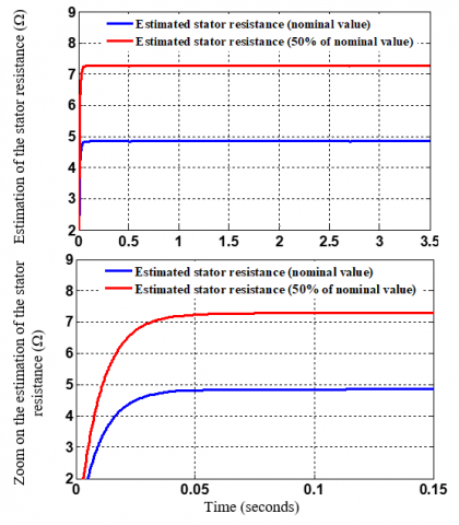
The Figure 4 shows the estimation of the stator resistance $\widehat{R}_{s}$ of the IM, with the nominal values of this machine 4.85 Ω, then for variations of + 50% on this value.
Figure 4. Estimation of stator resistance
The stator resistance estimation converges precisely. The estimated quantity reaches its actual value in less than 0.06 seconds after power-up.
The proposed control structure is implemented under MATLAB / SIMULINK environment, and tested under different operating conditions, in order to validate the performance of the DTC associated with the backstepping controller applied to the induction motor.
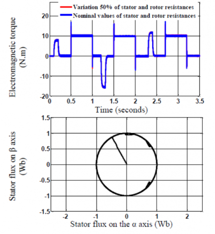
The Figure 5 shows the behavior of the system, at average speed, for the nominal values then with a variation of 50% of the stator and rotor resistances. The starting is fixed by a setpoint with a trapezoidal reference (+100 rd/s; -100 rd/s; +50 rd/s), followed by two successive reversals of rotation. Disturbances are introduced by application and suppression of a 10 Nm load torque. Figure 6 shows the behavior of the proposed drive, under low speed conditions, with a trapezoidal reference. The influence of the stator resistance being preponderant, the test is carried out with a 50% increase compared to its nominal value.
This test shows a high robustness, fast responding during the reversing state and accurate reference tracking in the steady state for Benchmark 1.
The employment of very low speeds is a necessary step to investigate control performance. Apparently, from the showing Figures 6 (Benchmark 2), the proposed DTC-Backstepping strategy preserves very acceptable operation with precise reference following and low speed fluctuation even at very low region (8 rad/s). This can prove the high capability of the combined Backstepping-nonlinear control law.
It can be seen that the stator current provided a good sinusoid and smooth waveform in both of simulation also and low harmonics. The flux trajectory is perfectly circular and the magnitude shows fast response and reduce ripples.
In the load application, it can be observed that the torque reduces ripples; moreover, the current shows good waveform in the load state also.
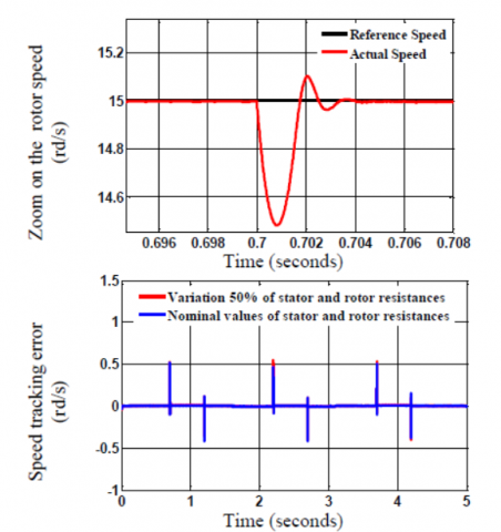
The Robustness test of parameter variation in the low speed region has conducted as a simulation study to check the ability of the proposed DTC-Backstepping technique while the variation of parameters. It consists of the variation of the stator and rotor resistance when the machine operates with a low speed (15rd/s and 8 d/s) and rated load. The Rs and Rr are increased by 50%.
The DTC-Backstepping proposed control which shows no considerable affection on the speed response and preserves an acceptable torque performance under these conditions.
Figure 5. Benchmark 1: Tracking trajectory and disturbance rejection performance of DTC-Backstepping approach
Figure 6. Benchmark 2: Tracking trajectory and disturbance rejection performance of DTC-Backstepping approach during low speed
In this work, the effects of the stator resistance variation on the performance of the DTC applied to IM is given. The variation of stator resistance deteriorates the performance of DTC drive particularly at low speed by introducing errors in electromagnetic torque and stator flux calculation. A super twisting stator resistance estimator is proposed, in order to cancel the influence resistive of the term. The simulation results show that the super twisting resistance estimator allows better tracking of the stator resistance change and improve the performance of DTC applied to the IM.
Then we presented the backstepping technique associated with the DTC to ensure a robust control against the various uncertainties and external disturbances and to improve some performance of the conventional DTC applied to the IM. The simulation results show that this combination of control gives better performance. Fast transient regimes are also noted, with a reduction in starting overrun and attenuation of torque, flux and current ripple.
This work is supported by the: Direction Générale de la Recherche Scientifique et du Développement Technologique (DGRSDT).
|
Tem,TL |
Electromagnetic torque, load torque |
|
$\dot{1}_{s \alpha}, \dot{1}_{s \beta}$ |
Stator currents |
|
$\mathrm{V}_{\mathrm{s} \alpha}, \mathrm{V}_{\mathrm{s} \beta}$ $\phi_{\mathrm{s} \alpha}, \phi_{\mathrm{s} \beta}$ |
Stator voltage Stator flux |
|
$\omega_{\mathrm{r}}$ |
Rotor speed |
|
$\sigma$ |
Total leakage factor |
|
$\mathrm{R}_{\mathrm{s}}$ and $\mathrm{R}_{\mathrm{r}}$ |
Stator and rotor resistances |
|
$\mathrm{L}_{\mathrm{s}}$ and $\mathrm{L}_{\mathrm{r}}$ |
Stator and rotor inductances |
|
Lm |
Mutual inductance |
|
p |
Pole pairs number |
|
J |
Total inertia of the system |
|
f |
Viscous damping coefficient |
|
$\mathrm{R}_{\mathrm{so}}, \hat{\mathrm{R}}_{\mathrm{s}}$ |
The nominal value and estimated stator resistance |
The induction machine nominal parameters:
\[\begin{align} & 1.5\text{ }kW,\text{ }3\text{ }phases{{,}_{{}}}50\text{ }Hz{{,}_{{}}}1420\text{ }rpm{{,}_{{}}}6.5/3.75\text{ }A,\text{ }4\text{ }poles,\text{ } \\ & {{R}_{s}}=4.85\text{ }\Omega ,\text{ }{{R}_{r}}=3.805\text{ }\Omega ,\text{ }{{L}_{s}}=0.274\text{ }H,\text{ }{{L}_{r}}=0.274\text{ }H,\text{ } \\ & {{L}_{m}}=0.258\text{ }H,\text{ }J=0.031\text{ }kg\cdot {{m}^{2}},\text{ }f=0.00114Nm\cdot s/rd. \\ \end{align}\]
[1] Mehazzem, F., Nemmour, A.L., Reama, A., Benalla, H. (2011). Nonlinear integral backstepping control for induction motors. In International Aegean Conference on Electrical Machines and Power Electronics and Electromotion, Joint Conference, Istanbul, pp. 331-336. https://doi.org/10.1109/ACEMP.2011.6490619
[2] Takahashi, I., Ohmori, Y. (2019). High-performance direct torque control of an induction motor. IEEE Transactions on Industry Application, 25(2): 257-264. https://dx.doi.org/10.1109/28.25540
[3] Ammar, A., Bourek, A., Benakcha, A., Ameid, T. (2017). Sensorless stator field oriented-direct torque control with SVM for induction motor based on MRAS and fuzzy logic regulation. 2017 6th International Conference on Systems and Control (ICSC), Batna, pp. 156-161. http://dx.doi.org/10.1109/ICoSC.2017.7958692
[4] Koratkar, P.J., Sabnis, A. (2017). Comparative analysis of different control approaches of direct torque control induction motor drive. In 2017 International Conference on Intelligent Computing, Instrumentation and Control Technologies (ICICICT), Kannur, pp. 831-835. http://dx.doi.org/10.1109/ICICICT1.2017.8342672
[5] Gedara, A.D., Ekneligoda, N.C. (2018). Direct torque control of induction motor using sliding-mode and fuzzy-logic methods. In 2018 IEEE Power & Energy Society Innovative Smart Grid Technologies Conference (ISGT), Washington, DC, pp. 1-5. http://dx.doi.org/10.1109/ISGT.2018.8403326
[6] Dannier, A., Pizzo, A.D., Noia, L.P.D., Meo, S. (2017). Integral sliding-mode direct torque control of sensorless induction motor drives. IEEE International Symposium on Sensorless Control for Electrical Drives (SLED), Catania, pp. 243-248. http://dx.doi.org/10.1109/SLED.2017.8078457
[7] Patel, D.N. (2017). Effect of change in stator sector region in direct torque control technique on induction motor. In 2017 International Conference on Energy, Communication, Data Analytics and Soft Computing (ICECDS), Chennai, pp. 2059-2062. http://dx.doi.org/10.1109/ICECDS.2017.8389811
[8] Xu, Y., Zhong, Y., Li, J. (2005). Fuzzy stator resistance estimator for a direct torque controlled interior permanent magnet synchronous motor. In 2005 International Conference on Electrical Machines and Systems, Nanjing, 1: 438-441. http://dx.doi.org/10.1109/ICEMS.2005.202564
[9] Lee, S.B., Habetler, T.G., Harley, R.G., Gritter, D.J. (2002). An evaluation of model-based stator resistance estimation for induction motor stator winding temperature monitoring. IEEE Transactions on Energy Conversion, 17(1): 7-15. http://dx.doi.org/10.1109/MPER.2002.4311669
[10] Ammar, A. (2019). Performance improvement of direct torque control for induction motor drive via fuzzy logic-feedback linearization. COMPEL-The International Journal for Computation and Mathematics in Electrical and Electronic Engineering, 38(2): 672-692. http://dx.doi.org/10.1108/COMPEL-04-2018-0183
[11] Babu, P.S., Ushakumari, S. (2011). Modified direct torque control of induction motor drives. 2011 IEEE Recent Advances in Intelligent Computational Systems, Trivandrum, Kerala, pp. 937-940. http://dx.doi.org/10.1109/RAICS.2011.6069446
[12] Youcefa, B.E., Massoum, A., Barkat, S., Wira, P. (2019), Backstepping direct power control for power quality enhancement of grid-connected photovoltaic system implemented with PIL co-simulation technique. Advances in Modelling and Analysis C, 74(1): 1-14. https://doi.org/10.18280/ama_c.740101
[13] Ammar, A. (2017). Improvement of direct torque control performances for asynchronous machine using non-linear techniques. Thesis, University Mohamed Khider, Biskra, Algeria.
[14] Chen, Y., Huang, S., Wan, S., Wu, F. (2007). A stator resistance compensator for a direct torque controlled low speed and high torque permanent magnet synchronous motor. In 2007 42nd International Universities Power Engineering Conference, Brighton, pp. 174-177. http://dx.doi.org/10.1109/UPEC.2007.4468941
[15] Haghbin, S., Zolghadri, M.R., Kaboli, S., Emadi, A. (2003). Performance of PI stator resistance compensator on DTC of induction motor. In IECON'03. 29th Annual Conference of the IEEE Industrial Electronics Society (IEEE Cat. No. 03CH37468), Roanoke, VA, USA, pp. 425-430. http://dx.doi.org/10.1109/IECON.2003.1280018
[16] Horch, M., Boumédiène, A., Baghli, L. (2018). Direct torque control for induction machine drive based on sliding mode controller with a new adaptive speed observer. In 2018 International Conference on Communications and Electrical Engineering (ICCEE), El Oued, Algeria, pp. 1-6. http://dx.doi.org/10.1109/CCEE.2018.8634546
[17] Goel, N., Patel, R.N., Chacko, S. (2015). A review of the DTC controller and estimation of stator resistance in IM drives. International Journal of Power Electronics and Drive Systems (IJPEDS), 6(3): 554-566. http://doi.org/10.11591/ijpeds.v6.i3.pp554-566
[18] Mashud, A., Bera, M.K. (2019). A multivariable super twisting sliding mode control of descriptor systems. In TENCON 2019-2019 IEEE Region 10 Conference (TENCON), Kochi, India, pp. 2663-2668. http://dx.doi.org/10.1109/TENCON.2019.8929361
[19] Li, Z., Zhou, S., Xiao, Y., Wang, L. (2019). Sensorless vector control of permanent magnet synchronous linear motor based on self-adaptive super-twisting sliding mode controller. IEEE Access, 7: 44998-45011. http://dx.doi.org/10.1109/ACCESS.2019.2909308
[20] Lascu, C., Argeseanu, A., Blaabjerg, F. (2019). Super-twisting sliding mode direct torque and flux control of induction machine drives. IEEE Transactions on Power Electronics, 35(5): 5057-5065. http://dx.doi.org/10.1109/TPEL.2019.2944124