Yongsheng Wang | Jing Gao* | Zhiwei Xu | Leixiao Li
© 2020 IIETA. This article is published by IIETA and is licensed under the CC BY 4.0 license (http://creativecommons.org/licenses/by/4.0/).
OPEN ACCESS
The output power prediction of wind power plants is an important guarantee to improve the utilization rate of wind energy and reduce wind curtailment. However, due to the strong randomness of wind energy, the ultra-short-term prediction accuracy of wind power output is poor. In view of the problem above, a prediction model based on deep learning of grouped time series (LW-CLSTM) was proposed in this paper. Based on this model, the authors attempted to explore a prediction method of wind power output. For this, first the multivariate data of wind power was fused, cleaned, dimension-reduced, and standardized, and the time period characteristics of the output power itself were extracted. Afterwards, it proposes a time sliding window (TSW) algorithm, and constructs a neural network input data set. Then a deep neural network prediction model combining the Convolutional Neutral Network (CNN) and Long-Short Term Memory (LSTM) was established, and the regression evaluation criteria for output power forecast accuracy in wind power production were designed, to compare the proposed model with four other prediction models. Finally, the experiments on the TensorFlow platform using real data show that this model has better prediction accuracy than the other four models, reaching a prediction accuracy rate of 92.5%, which verified the effectiveness of this prediction method.
wind power plant, output power prediction, short-term wind power prediction, deep learning, new energy application
As an important renewable energy source, wind energy has developed rapidly in recent years. Due to its characteristics of randomness and fluctuation, the wind output power is unstable. Also, large-scale wind power access poses challenges to the normal operation, scheduling and grid security of power systems [1-3]. The forecast technology of wind power output provides a method to solve this problem. It can predict the output power of wind power plants in the future, and is of great significance in formulating a reasonable dispatching and maintenance plan, and improving wind power utilization [4-7].
The research on wind power output prediction has been carried out for decades, achieving a wealth of research results. According to the length of forecast time, wind power output forecast can be divided into ultra-short-term forecast, short-term forecast, and medium- and long-term forecast [8, 9]. Ultra-short-term forecasts focus on active output power within 30 minutes to 4 hours, short-term forecasts focus on that within 1 to 3 days, and medium- and long-term forecasts focus on that in the coming weeks, months, and years. In terms of the differences in wind power forecast technologies, there have formed several types of stable wind power output forecast methods [10], namely physical model method [11], conventional statistical model method [12], and intelligent calculation method [13]. First, the physical model method uses numerical weather prediction (NWP) data to obtain microscale meteorological information by performing terrain, wake flow, and spatial correlation analysis on the surrounding area of the wind farm, and then combines the technical parameters of the wind turbine and the energy conservation equation to achieve its output power. This method is suitable for medium and long-term prediction, but excessive empirical parameters lead to the complexity of the model, the large amount of calculation and the difficulty of transplantation. Second, the conventional statistical model method usually uses the wind power time series and wind speed time series as the basis. It can establish the mapping relationship between the input characteristics and the wind power time series only through the historical data. After performing statistical regression fitting of various historical meteorological data and power data, this method shall realize the prediction of future output power. Specifically, the commonly used methods include Kalman filter method [14], random time series method [15, 16], support vector machine method [17, 18], and so on. Literatures [19-21] have successfully used statistical model methods in short- and medium-term wind power prediction. However, the conventional statistical model is difficult to construct, with strong randomness of parameters, and the accuracy of prediction cannot be guaranteed. The third is the intelligent calculation method. With the in-depth development of computer software and hardware technology, and artificial intelligence theory, wind power forecasting has gradually begun to use the intelligent calculation, such as wavelet analysis prediction method, genetic algorithm prediction and other prediction algorithms. These algorithms use different structural designs to extract different features of the data. But they vary greatly in terms of the principles, making it difficult to build models, and the prediction results still cannot fully meet the actual requirements of wind power companies.
With the deep development of machine deep learning theory, researchers have attempted to use deep learning methods in intelligent computing. Deep neural networks can effectively avoid the disappearance of gradients [22-24]. Its multilayer network structure can fit complex non-linear mappings, and has obvious advantages when processing large numbers of samples and non-linear data. Also, its prediction results are reproducible, saving the computing resources of the wind power prediction system [25, 26]. Deep neural networks [27], Convolutional Neural Networks (CNN), and Recurrent Neural Network (RNN), etc. are often applied in deep learning. Literatures [28, 29], based on the GRU and CNN (improved version of the LSTM), have made some progress in building a combined deep learning network. However, there are various influencing factors on the wind power prediction problems, and most of them are continuous variables, which leads to an exponential increase in the computational complexity of many network parameters when directly input in deep learning network. Without scientific and reasonable optimization, it shall result in low accuracy of network prediction poor generalization ability, and even the difficulty for the network to converge.
This paper mainly studies the short-term and ultra-short-term output power prediction of wind power from several hours to several days. For this, it proposes to build a prediction model (LW-CLSTM) based on deep learning of grouped time series. This model performs multivariate data fusion of historical wind power data, historic metrological data, and turbine state data, construction of time series data sets with the TSW, extraction of time cycle characteristics of wind power output, and establishment of deep networks using CNN and LSTM network structures. Then, a prediction method with high prediction accuracy and strong operability was formed through the multivariate data fusion, data cleaning, construction of deep learning models, and improvement in the evaluation criteria. Finally, the experiments were conducted on this method using the real data, to obtain 92.5% of accuracy based on the evaluation indicators of d_MAE average difference method (see 2.6.2).
2.1 Overall framework of wind power output prediction method
The wind power prediction process includes raw data collection of wind farm, data fusion and cleaning, data dimensionality reduction and standardization, construction of data sets, establishment of CNN-LSTM deep learning models, training and optimization of models, prediction and evaluation. The output power prediction of a wind power plant is essentially a problem of mapping a set of input sequences to a set of output sequences. Its core is how to generate a predicted power sequence.
Figure 1. Flow chart of wind power output prediction
The prediction process is divided into six stages (Figure 1): (1) Multivariate data fusion and cleaning. Collect the meteorological data, historical power data and wind turbine status data of the wind farm, perform the unification of data format and time intervals, and splice the data in the corresponding sampling time, fill in missing values and correct distortion values; (2) Data dimension reduction and standardization. The data is subjected to standardized processing such as dimensionality reduction, discretization, normalization, and one-hot encoding to form discrete data including only 0 and 1. (3) Construction of data sets using the sliding window. Analyze the time period characteristics of the data, and propose to use the TSW to construct a grouped time series data set and extract the grouping time series characteristics of the data; (4) Establishment of a deep learning model. Based on the TSW data set, a multi-layer CNN and LSTM network structure are combined to establish a deep learning model (LW-CLSTM) and realize automatic extraction of wind power features; (5) Model training and optimization. Use the real data set to train the deep combination model, and optimize the model based on the test data set; (6) Model evaluation and prediction. The trained model is used for prediction, and compared with the actual output power data and other prediction methods.
2.2 Data fusion and cleaning
There are many types of data generated by wind power plants, e.g., the volume of some data is huge, formats and time intervals of some other data are inconsistent, and abnormal data such as missing data and distortion also exist. All these data related to each other contain the key factors for the normal operation of wind turbines [30], which requires data fusion and cleaning.
Data fusion is to unify the time intervals according to the sampling frequency of 15 minutes, and then perform data splicing in the corresponding sampling time, so that the data is presented in the form of a unified two-dimensional table and form an initial two-dimensional data set. Data cleaning means to deal with missing values and distortion values. The missing value in wind power data is the time series where the output power is located. It will destroy the original data structure to continuously or randomly distribute it in the middle of the data, or directly delete or simply complete (zero value completion, before and after value completion, and mean value completion). Given that only the output power sequence is missing in the fused data set, it is a univariate data missing problem. Thus, this paper uses a multiple linear regression method to predict missing values in the data sequence. For the distortion value in the data, t test can be first used to find and delete it directly, and then correct it according to the processing method of missing values.
2.3 Data dimension reduction and standardization
Through data fusion and cleaning, the initial data set is obtained. It includes various features of different types of data mentioned above, most of which have little effect on wind power output power. In order to reduce the amount of calculation and facilitate the network convergence, the data is reduced in dimension. In this paper, Principal Component Analysis (PCA) was used for feature selection and data dimension reduction. However, there are still significant differences in the dimension of various features retained after the PCA. To ensure the fair contribution of each variable to the machine learning result, each variable is normalized and converted into a relative amount with unified dimension. Due to the continuous features of the normalized data, segmented discretization and one-hot encoding can be performed to make the final data set appear as a three-dimensional sparse matrix with only 0 and 1, which can greatly reduce the amount of network calculation and speed up network convergence.
2.4 Construction of input data set based on time sliding window
To mine all the features of the initial wind power data, an algorithm based on the TSW was proposed to construct the input data set and expand the input data, thereby improving the prediction accuracy. The actual output power is sequence data with a time period. Extracting its period characteristics can improve the prediction accuracy of the model. Therefore, the actual output power was added to the DATA set of the input data set.
Figure 2. Construction diagram of training data set using the time sliding window
Figure 2 shows the construction of the training data set using a sliding window. The periodic characteristics of the actual output power data were analyzed to determine the lookback of the sliding window. By moving the window downwards, the standard data was segmented to form the input sample set. When selecting data in a sliding window, the first sample was the first to the lookback records of the data, the second sample was the second to the lookback +1 records, and so on. Let the total number of data records be L, then the number of records in the data set constructed by the sliding window was (L-lookback+1)×lookback, which is equivalent to the original data being expanded by lookback times.
2.5 Establishment of a deep network model based on the CNN and LSTM
Considering the significant periodicity of wind power data, RNN can be used to extract time-period features, while CNN can quickly and automatically extract local features and significantly reduce the amount of calculations. Therefore, based on these two network structures, this paper attempts to build a combined neural network model for wind power prediction.
2.5.1 LSTM-BASED Extraction of time series features
The normalized data set is a time series, and the predicted output power data is a time period series. The RNN can be used to construct a deep learning model, which can process end-to-end sequence data. But when the input time sequence or the time series to be predicted is long, the historical sequence information will be replaced by the more recent information, causing the far-end information obtained by the RNN training to disappear or explode. Thus, the RNN is not suitable for processing time series data. LSTM network is an improvement of RNN. This block adds four structures: input gate, output gate, forget gate, and memory cell while retaining the advantages of standard RNN network structure. This can achieve reasonable retention and forgetting of grouped time series state of wind power, eliminate the problem of gradient disappearance or local optimization, and has a good memory effect on wind power output and time period characteristics of historical meteorological data, thereby achieving higher prediction accuracy in theory [31, 32]. Figure 3 shows the abstract structure of the hidden layer in LSTM.
Figure 3. LSTM network structure
In Figure 3, when the time step is t (t=1, 2 ..., n), then the input state of the LSTM block is xt, the forget gate state is ft, the input gate state is it, the output gate state is Ot, while the unit candidate state signal is $\tilde{N}_{t}$, the unit memory state is Nt, and the unit output state is ht. The forget gate controls the wind power information that is forgotten; the input gate processes the signals received by the unit to generate signals it and candidate signals $\tilde{N}_{t}$, and also updates the state of the unit Nt; the output gate generates signals and determines the output signal ht of the unit. The signal conversion between units can be expressed as:
${{f}_{t}}=\text{ }\!\!\sigma\!\!\text{ }\left( {{W}_{\text{f}}}\cdot \left[ {{\text{h}}_{\text{t}-1}},{{\text{x}}_{\text{t}}} \right]+{{\text{b}}_{\text{f}}} \right)$ (1)
${{\text{i}}_{\text{t}}}=\text{ }\!\!\sigma\!\!\text{ }\left( {{\text{W}}_{\text{i}}}\cdot \left[ {{\text{h}}_{\text{t}-1}},{{\text{x}}_{\text{t}}} \right]+{{\text{b}}_{\text{i}}} \right)$ (2)
${{\text{ }\!\!\tilde{\mathrm{N}}\!\!\text{ }}_{\text{t}}}=\tanh ({{\text{i}}_{\text{t}}}\left( {{\text{W}}_{\text{C}}}\cdot \left[ {{h}_{\text{t}-1}},{{\text{x}}_{\text{t}}} \right]+{{\text{b}}_{\text{C}}} \right)$ (3)
${{\text{N}}_{\text{t}}}={{\text{f}}_{\text{t}}}\cdot {{\text{N}}_{\text{t}-1}}+{{\text{i}}_{\text{t}}}\cdot \widetilde{{{N}_{t}}}$ (4)
$\mathrm{o}_{t}=\sigma\left(W_{o} \cdot\left[\mathrm{H}_{\mathrm{t}-1}, \mathrm{x}_{\mathrm{t}}\right]+\mathrm{b}_{o}\right)$ (5)
${{\text{h}}_{\text{t}}}={{\text{O}}_{\text{t}}}\cdot \text{tanh}\left( {{\text{N}}_{\text{t}}} \right)$ (6)
It can be seen that the time periodic characteristics of wind power sequence data can be memorized for a long time in each node of the LSTM network. Information that needs to be forgotten can also be completed by the cell forgetting mechanism. After multiple input training, the LSTM deep network can well fit the non-linear relationship between input data and output power data of wind power, and obtain satisfactory prediction results.
2.5.2 CNN-based fast extraction of features
Due to the long time span of wind power sequence data and much time required for model training, CNN can be used to optimize the model and shorten the training time. 1D CNN is very applicable to time series data analysis, and suitable for analyzing signal data with a fixed length period.
Figure 4. Schematic diagram of 1D CNN convolution
Figure 4 shows the convolution principle of a filter's 1D CNN on the wind power sequence data. For the standardized wind power sequence data, each element is a two-dimensional matrix with a width as the feature number and a height as the TSW value (LookBack). Taking the size of the filter's convolution kernel as Height, then each convolution forms a convolution window with a width of Feature and a height of LookBack, and then convolves downwards until the end. The 1D CNN convolution filter is a one-dimensional vector, which does not change the number of features. It can only reduce the vertical LookBack value through the convolution operation to obtain a new time window value NewStep as shown in (7), which reduces the amount of calculation while automatically extracting features locally.
$\text{NewStep=(Loo}kBack-Height+1)\times N$ (7)
Figure 4 shows the convolution process of a filter, but a convolution filter can only learn one feature. In order to comprehensively learn the features of wind power sequence data, N convolution filters are defined. After one convolution, a two-dimensional matrix NewStep´N is derived as the output of the first convolution. The output data of multiple convolutions can be pooled to further reduce the data dimension and increase the operation speed.
2.5.3 Establishment of a combined neural network model based on CNN and LSTM
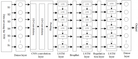
As above, this paper established the deep learning model using the CNN and LSTM combined network based on the TSW data set. The prediction model is composed of a data input layer, two convolution layers, two dense layers, three LSTM layers, and DropOut layer.
Figure 5. Network structure of the LW-CLSTM prediction model
Figure 5 shows the structure of the prediction model. It consists of dense layers (fully connected), CNN convolution layers, LSTM layers and output layer. The data processing in this network structure is as follows:
(1) The TSW data set was input into a dense layer. The data set was a three-dimensional matrix X; the first dimension of X was the number of elements of the two-dimensional matrix determined by the total data sample and time window size; each element was a two-dimensional matrix with the number of rows as the size of the time window and the number of columns as the feature number of input data. The number of elements and the number of features in the dense layer were the same. This layer passed all the characteristics of the input data to the next layer;
(2) The convolution layer received the output of the dense layer, and output a two-dimensional matrix $\text{NewStep}\times N$ through two layers of convolution and one layer of pooling. At this time, the features of the wind power sequence data were automatically extracted, but the time window value of the data has been reduced three times, and the amount of data also decreased simultaneously;
(3) Then, the LSTM layer was composed of three LSTM layers, one DropOut layer, and one regularization layer. Each layer of LSTM consisted of 32, 64, and 96 LSTM cells, and this layer automatically extracted the correlation between meteorological data and output power, and data time-order characteristics; regularization layer and DropOut layer prevent overfitting in training between the two LSTM layers;
(4) Finally, the network output a predicted power sequence through a dense layer.
2.6 Evaluation index design for regression prediction accuracy of LW-CLSTM model
Error evaluation standards such as mean absolute error (MAE), and R2-Score, etc. are commonly used in regression analysis [33, 34], but for wind power plants, statistical evaluation criteria for prediction accuracy need to be designed. This paper designs two evaluation standards: the statistical distribution method of maximum relative error (s_MRE), and the MAE average difference method (d_MAE).
2.6.1 Statistical distribution method of maximum relative error s_MRE
In addition to the evaluation criteria such as the mean square error (MSE), root mean square error (RMSE), MAE, and R2-Score commonly used in regression analysis, this paper also designs an intuitive evaluation standard of regression prediction accuracy s_MRE based on the statistical distribution of predicted and true values, as shown in formula (8). Let the number of test sets be N, the ratio of the absolute value to the true value of the difference between the i-th predicted value and the true value in the test set be λi; let the acceptable value λi of the power plant be θ, and the number of the predicted values in the test set that satisfy λi<θ be n, then (n/N)% was the statistical accuracy rate A of the prediction model. After joint research with the wind power plant, the value of θ that met the production needs was 0.2, the accuracy of the model constructed could reach up to 755, and the corresponding R2-Score value was 0.93.
$\lambda_{i}=\frac{\left|y_{i}-\widehat{y_{i}}\right|}{y_{i}}, n=\sum_{i=1}^{n} \lambda_{i} \leq \theta$, $A=\left\{\frac{\sum_{i=1}^{n}\left[\frac{\left|y_{i}-\widehat{y_{i}}\right|}{y_{i}}\right] \leq \theta}{N}\right\} \%=\left(\frac{n}{N}\right) \%$ (8)
In formula (8), $\lambda_{i}$ is the relative error. The value of A is obtained under the maximum tolerable relative error, which is the error evaluation method proposed in this paper.
2.6.2 Mean difference method d-MAE
In order to meet the requirements of forecasting accuracy evaluation during wind farm operation, this paper also design a mean error difference method, as shown in formula (9) in this paper. The value size is positively correlated with the prediction accuracy.
$\mathrm{d}_{-} \mathrm{MAE}=1-\frac{\frac{1}{n} \sum_{i=1}^{n}\left|y_{i}-\widehat{y_{i}}\right|}{\widehat{y_{i}}}=1-\frac{\mathrm{MAE}}{\bar{y}}$ (9)
This experiment used Keras deep learning platform with TensorFlow as the underlying layer. It called data processing and data visualization modules such as NumPy for data processing and display, the optimizers module for optimization of error back propagation, the regularizers module for regularization of the model, the callbacks module for dynamic adjustment of the learning rate, and CNN1D and LSTM modules to build a long-term and short-term memory deep learning model based on a TSW data set. Besides, Python was applied to write programs, and the experimental environment was a GPU deep learning platform.
3.1 Experimental data set
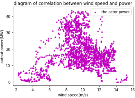
Experimental data were collected from a wind farm of certain wind power company in Inner Mongolia for model training and verification. They were mainly divided into two parts: the first part was the numerical weather prediction data, from January 1, 2019 to May 22, 2019, for a total of 13,632 records, which included 9 fields such as date and time etc. The other part was the output power data from January 1, 2019 to May 21, 2019, for a total of 13,536 records. After the data splicing, the PCA was performed to finally obtain 13,494 valid records with 7 characteristics such as wind speed and output power, which constituted the initial data set. Intuitively, the output power and wind speed should be linearly related. To verify this, a scatter plot was drawn for correlation analysis as shown in Figure 6. It can be seen from the figure that there is no simple linear relationship between wind speed and output power, and a deep learning model needs to be established, enabling the machine automatically to learn its complex non-linear relationship.
Figure 6. The scatter plot of wind speed and direction
3.1.1 Periodic analysis of data
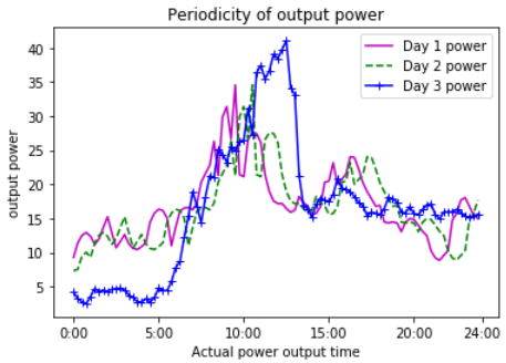
Periodical analysis was conducted on the actual power data in the initial data set. In the experiment, the sample data were visually displayed for three consecutive days from 00:00 to 24:00 every day, including a total of 96 sampling records for 24 hours (Figure 7). It is found from the figure that the output power of three consecutive days has a periodic characteristic of phase equity, indicating that the periodic characteristic of the output power itself should be extracted to improve the prediction accuracy.
3.1.2 Construction of an input data set using time sliding window
In order to extract the time periodic characteristics of the output power itself, the output power combined with other meteorological data was taken as input features, and the data set was divided into a Data set and a Label set; the Data set was a two-dimensional matrix of 13,494 rows and 7 columns, and the Label set was One-dimensional matrix of 13,494 elements. Referring to the periodic analysis of the data, the TSW value Lookback was selected to be 288. To construct the data set using the sliding window described above, the final shape of the Data set was (13206,288,7), and that of the Label set was (13206,1). Then the data was standardized and discretized to ensure that it contains only 0 and 1 in the form of sparse matrix. Finally, dividing the processed data set into training and test sets, the data set was constructed.
Figure 7. Periodicity of actual output power
3.2 Error evaluation index
MSE, RMSE, MAE and R2-score are commonly used for evaluation in regression analysis. RMSE is the root of MSE; it’s better to obtain a smaller value for both in the same data set, but the data set size is sensitive. MAE is not affected by the size of the data set, and can better reflect the actual situation of the prediction error. RMSE and MAE have a good error evaluation function under the same data set, but due to different dimensions, it is difficult to measure the effectiveness of the model. R2-score can eliminate the effects of different dimensions through average calculation; in practice, the value of R2-score is closer to 1, with a better model effect. This paper uses the MAE indicator in the loss curve of the prediction model, and compares the performance of different prediction models on the above indicators in the experiments.
3.3 Experimental design
3.3.1 LW-CLSTM model experiment
A TensorFlow-based Keras deep learning platform was deployed on the GPU platform. According to the designed model, a deep network was built, which consists of a dense (fully connected) input layer, the hidden layer (incl. two CNN convolutional layers, a maximum pooling layer, three LSTM layers, and three DropOut layers), and an output layer. The network involves different categories of hyper-parameters: the number of nodes in the input layer, the number of nodes in each LSTM layer, L1\L2 regularization parameters, DropOut automatic drop index, gradient optimizer Nadam's initial parameters and automatically decreasing parameters of learning rate. Table 1 shows the setting of each hyper parameter.
3.3.2 Comparative experiment design
In order to compare and evaluate the prediction effect of the LW-CLSTM model, a TLW-LSTM model was designed by removing the CNN convolution layer based on the LW-CLSTM model. Meanwhile, several types of machine learning models such as support vector machines, decision trees, and random forests were designed for comparative evaluation.
Table 1. Hyper parameters of deep neutral network
|
Parameter type |
Node number |
Convolution kernel |
Pooling kernel |
Activation function |
L1 regularization |
L2 regularization |
DropOut |
Optimizers |
|
Input layer |
7 |
- |
- |
RELU |
- |
- |
- |
- |
|
CNN1 |
32 |
3 |
- |
RELU |
- |
- |
- |
- |
|
CNN2 |
32 |
3 |
- |
RELU |
- |
- |
0.3 |
- |
|
MaxPooling |
- |
- |
4 |
- |
- |
- |
- |
- |
|
LSTM1 |
32 |
- |
- |
Sigmod |
0.001 |
0.002 |
0.3 |
Nadam |
|
LSTM2 |
64 |
- |
- |
Sigmod |
0.001 |
0.001 |
0.5 |
Nadam |
|
LSTM3 |
64 |
- |
- |
Sigmod |
0.001 |
0.002 |
0.6 |
Nadam |
|
Nadam |
Lr=0.002, Beta_1=0.9, Beta_2=0.999, Epsilon=1e-08, Schedule_decay=0.004 |
|||||||
|
Reduce_lr |
Patience=5, Factor=0.8, Mode='auto', Verbose=1, Min_delta=0.0001, Cooldown=0, Min_lr=0.0000001 |
|||||||
3.4.1 Experimental analysis of LW-CLSTM and TLW-LSTM models
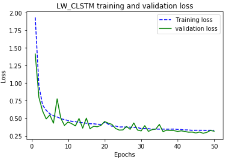
The processed training data set was used to perform 50 rounds of iterative training on the constructed LW-CLSTM model, and draw the MAE loss curve of the training process as shown in Figure 8 (a). It can be seen from the figure that the losses of training and testing at the beginning were decreased rapidly, and then started to decline slowly after 5 rounds; after 30 rounds, the trained MAE and MAE also decreased slowly; after 50 rounds, the loss reached the lowest level and the model completely converged. In contrast, as shown in Figure 8 (b), the TLW-LSTM had no convolutional layer, but the performance of the training loss curve was basically the same, indicating that the CNN convolution and pooling have no significant effect on the loss of the model, and the network convergence of the two is basically synchronous.
(a) The loss curve of LW-CLSTM model
(b) The loss curve of TLW-LSTM model
Figure 8. Comparison of training loss curves between LW-CLSTM and TLW-LSTM models
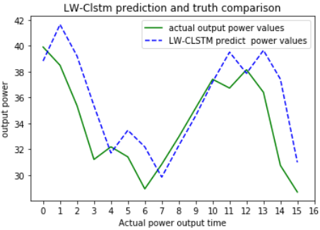
The trained model was applied to predict the output power of the input data of the test set, which were then compared with the actual power data of the test set. Figure 9 shows the comparison curve of the predicted power and actual output curve of the two models within 4 hours. The horizontal axis was the sampling time at 15 minute intervals, and the vertical axis was the megawatt (MW) power value. It can be seen from Figure 9 that the predicted power curves of the two models well fit the actual output power curves of the wind farm. To compare the convergence time of the two models under the same data set, after 50 rounds of training, the TLW-LSTM spent 80 minutes, and the average time per round was 96 seconds, while the LW-CLSTM model need 25 minutes, and 29 seconds per round. This indicates that the CNN network greatly reduces the amount of calculation and accelerates the training speed without affecting the accuracy of LSTM training.
(a) Training accuracy curve of LW-CLSTM model
(b) Training accuracy curve of TLW-LSTM model
Figure 9. Comparison of predicted power and actual power between LW-CLSTM and TSW-LSTM model
3.4.2 Comparative analysis of experiments
In order to better reflect the engineering value of the model constructed in this paper, a random forest learning model was also designed in the experiment to compare with the deep learning model proposed. All models were experimentally verified under the same data set, and the output power within the next 24 hours was predicted. The error index of each model is shown in Table 2 and Figure 10.
Table 2. Comparison of errors and accuracy indicators between various prediction models
|
Evaluation indicators |
MSE |
RMSE |
MAE |
R2-Score |
d_MAE |
s_MRE |
|
Physical model |
220.1 |
149 |
8.53 |
- |
65.7% |
56.3% |
|
Random forest |
1162.2 |
34.0 |
19.12 |
0.41 |
61.4% |
38.6% |
|
TLW-LSTM |
11.7 |
3.4 |
1.39 |
0.93 |
92.7% |
77.9% |
|
LW-CLSTM |
12.7 |
3.5 |
1.36 |
0.93 |
92.5% |
75.7% |
The MAE value of the LW-CLSTM prediction model constructed in this paper was 1.36, and the d_MAE value was about 92% which is significantly better than the other two models; the s_MRE value was 76%, indicating that the prediction result is highly recognized by users. In addition, LW-CLSTM and TLW-LSTM have basically the same performance in various evaluation indicators such as accuracy and error, which shows that after CNN convolution and pooling are added to the TLW-LSTM model, features can still be extracted well, and the operation speed is accelerated.
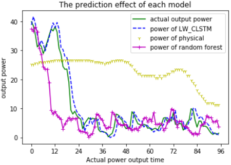
Figure 10. Comparison of prediction effects between different models
Figure 10 compares the power curves of the physical model, the LW-CLSTM model, and the random forest model and the actual output power curve. The predicted output power curve of the physical model and the random forest within a day differs significantly from the actual output power curve, and both curves cannot fit synchronically. The output power curve predicted by the LW-CLSTM method proposed in this paper fits well with the actual output power curve within a day, and has obtained higher prediction accuracy.
This paper conducts an experimental study on the whole process of short-term and ultra-short-term wind power prediction including data processing, prediction model construction, prediction effect evaluation, and model optimization. It proposes to fuse the time period characteristics of historical power data and use sliding time windows for constructing the input data sets, and then constructs an LW-CLSTM deep learning model for wind power prediction. In addition, two kinds of regression evaluation criteria for wind power prediction were designed using real wind farm data. Finally, the proposed model was compared with other models, to verify its good prediction accuracy. The following conclusions have been drawn:
(1) It can effectively extract the time periodic characteristics of the output power and improve the prediction accuracy rate by integrating the historical power data into the input data set, and using the TSW;
(2) The use of LSTM effectively extracts the time series characteristics of the data set, fit the output power curve of the wind farm well, and obtain good prediction results;
(3) The use of CNN convolutional network can significantly reduce the training time of the model, and improve its practicability, thereby verifying the effectiveness of the proposed prediction method in this paper.
This work is supported by Inner Mongolia Science and Technology Major Special Projects (Research And Development of Cloud Computing Application Technology); Natural Science Foundation of China (61462070, 61962045, 61502255, 61650205); Inner Mongolia Agricultural University Doctoral Scientific Research Fund Project (NO.BJ09-44); Natural Science Foundation of Inner Mongolia Autonomous Region (2018MS06003, 2017MS(LH)0601, 2019MS06027); Inner Mongolia Key Technology Research Plan Project (Toward Big Data Storage and Mining Platform for Intelligent Transportation); Major Special Project of Science and Technology in Inner Mongolia Autonomous Region (Development and Application of Private Cloud Operating System Based on OpenStack).
[1] Ding, M., Zhang, C., Wang, B., Bi, R., Miao, L.Y., Che, J.F. (2019). Short-term forecasting and error correction of wind power based on power fluctuation process. Automation of Electric Power Systems, 43(3): 2-12. https://doi.org/10.7500/AEPS20180322011
[2] Zhang, Y.T., Wang, Z.Y., Lei, Y.F., Wu, D.S., Cheng, R.L., Hua, D. (2019). An evaluation method for the maximum penetration of wind power of district power grid based on the self-organization criticality. Power System Protection and Control, 47(2): 9-15. https://doi.org/10.7667/PSPC201863
[3] Costa, A., Crespo, A., Navarro, J., Lizcano, G., Madsen, H., Feitosa, E. (2008). A review on the young history of the wind power short-term prediction. Renewable and Sustainable Energy Reviews, 12(6): 1725-1744. https://doi.org/10.1016/j.rser.2007.01.015
[4] Liu, S.W. (2016). Study on the influence mechanism of grid-connected doubly-fed wind turbine on transient stability of power system. North China Electric Power University.
[5] Mu, G., Yang, M., Wang, D., Yan, G., Qi, Y. (2016). Spatial dispersion of wind speeds and its influence on the forecasting error of windpower in a wind farm. Journal of Modern of Power Systems and Clean Energy, 4(2): 265-274. https://doi.org/10.1007/s40565-015-0151-x
[6] Soder, L., Hofmann, L., Orths, A., Holttinen, H., Wan, Y., Tuohy, A. (2007). Experience fromwind integration in some high penetration areas. IEEE Trans on Energy Conversion, 22(1): 4-12. https://doi.org/10.1109/TEC.2006.889604
[7] Li, J., Yu, Y. (2018). Short-term wind power time series prediction based on sparse coding method. Power System Protection and Control, 46(12): 16-23. https://doi.org/10.7667/PSPC170765
[8] Han, S. (2008). Research on short-term prediction method of wind farm power. North China Electric Power University (Beijing).
[9] Miao, N. (2014). Research on short-term prediction of wind power of wind speed. Shandong University.
[10] Han, Z.F., Jing, Q.M., Zhang, Y.K., Bai, R.Q., Guo, K.M., Zhang, Y. (2019). Review of wind power forecasting methods and new trends. Power System Protection and Control, 47(24): 178-187.
[11] Chen, Y., Zhou, H., Wang, W.P., Cao, X., Ding, J. (2011). Improvement of Ultra-short-term Forecast for Wind Power. Automation of Electric Power Systems, 35(15): 30-33, 87.
[12] Alexiadis, M.C., Dokopoulos, P.S., Sahsamanoglou, H.S., Manousaridis, I.M. (1998). Short-term forecasting of wind speed and related electrical power. Solar Energy, 63(1): 61-68. https://doi.org/10.1016/S0038-092X(98)00032-2
[13] Brown, B.G., Katz, R.W., Murphy, A.H. (1984). Time-series models to simulate and forecast wind-speed and wind power. Journal of Climate and Applied Meteorology, 23(8): 1184-1195. https://dx.doi.org/10.1175/1520-0450(1984)023%3C1184:TSMTSA%3E2.0.CO;2
[14] Yu, C., Xue, Y.S., Wen, F.S., Dong, Z.Y., Wong, K.P., Li, K. (2015). An ultra-short-term wind power prediction method using 'Offline classification and optimization, Online model matching' based on time series features. Automation of Electric Power Systems, 39(8): 5-11. https://doi.org/10.7500/AEPS20141230007
[15] Lee, D., Baldick, R. (2014). Short-term wind power ensemble prediction based on Gaussian processes and neural networks. IEEE Transactions on Smart Grid, 5(1): 501-510. https://doi.org/10.1109/TSG.2013.2280649
[16] Li, Z., Han, X.S., Han, L., Kang, K. (2010). An ultra-short-term wind power forecasting method in regional grids. Automation of Electric Power Systems, 34(7): 90-94.
[17] Liu, A.G., Xue, Y.T., Hu, J.L., Liu, L.P. (2015). Ultra-short-term wind power forecasting based on SVM optimized by GA. Power System Protection and Control, 43(2): 90-95. https://doi.org/10.7667/j.issn.1674-3415.2015.02.014
[18] Ding, Z.Y., Yang, P., Yang, X., Zhang, Z. (2012). Wind power prediction method based on sequential time clustering support vector machine. Automation of Electric Power Systems, 36(14): 131-135, 149. https://doi.org/10.3969/j.issn.1000-1026.2012.14.025
[19] Guo, C.X., Wang, Y., Shen, Y., Wang, M., Cao, Y.J. (2012). Multivariate local prediction method for short-term wind speed of wind farm. Proceedings of the CSEE, 32(1): 24-31.
[20] Li, J., Yu, Y. (2018). Short-term wind power time series prediction based on sparse coding method. Power System Protection and Control, 46(12): 16-23. https://doi.org/10.7667/PSPC170765
[21] Liu, C.L., Cao, W., Wang, Z.Q. (2019). Short-term interval prediction of wind power based on fuzzy C-means soft clustering condition identification. Journal of North China Electric Power University (Natural Science Edition), 46(5): 83-91.
[22] Maragatham, G., Devi, S. (2019). LSTM model for prediction of heart failure in bigdata. Journal of Medical Systems, 43: 111. https://doi.org/10.1007/s10916-019-1243-3
[23] Bengio, Y., Ducharme, R., Vincent, P., Jauvin, C., Kandola, J., Hofmann, T., Poggio, T., Shawe-Taylor, J. (2003). A neural probabilistic language model. Journal of Machine Learning Research, 3(6): 1137-1155. https://doi.org/10.1162/153244303322533223
[24] Lee, H.Y., Tseng, B.H., Wen, T.H., Tsao, Y. (2017). Personalizing recurrent-neural-network-basedlanguage model by social network. IEEE/ACM Transactions on Audio, Speech, and Language Processing, 25(3): 519-530. https://doi.org/10.1109/TASLP.2016.2635445
[25] Zhao, Z.H., Zhang, J.S., He, P.D., Yang, K.L., Wang, C.C. (2019). Wind power prediction based on wide and deep neural network. Journal of China Academy of Electronics and Information Technology, 14(3): 307-311. https://doi.org/10.3969/j.issn.1673-5692.2019.03.015
[26] Cui, M.J., Sun, Y.Z., Ke, D.P. (2014). Wind power ramp events forecasting based on atomic sparse decomposition and bp neural networks. Automation of Electric Power Systems, 38(12): 6-11. https://doi.org/10.7500/AEPS20130418003
[27] Zhu, Q.M., Li, H.Y., Wang, Z.Q. (2017). Short-term wind power forecasting based on LSTM. Power System Technology, 41(12): 3797-3802. https://doi.org/10.13335/j.1000-3673.pst.2017.1657
[28] Xue, Y., Wang, L., Wang, S., Zhang, Y.F., Zhang, N. (2019). An ultra-short-term wind power forecasting model combined with CNN and GRU networks. Renewable Energy Resources, 37(3): 456-462. https://doi.org/10.3969/j.issn.1671-5292.2019.03.023
[29] Yang, M., Sun, Y., Sun, Z.J., Yin, Y.L., Han, J.F. (2014). Design and development of large-scale data management system of wind farm. Journal of Northeast China Institute of Electric Power Engineering, 34(2): 27-31. https://doi.org/10.3969/j.issn.1005-2992.2014.02.006
[30] Wang, C., Zhang, H.L., Fan, W.H. (2018). Wind power prediction based on projection pursuit principal component analysis and coupling model. Acta Energiae Solaris Sinica, 39(2): 315-323.
[31] Qian, Y.S., Shao, J., Ji, X.X., Li, X.R., Mo, C., Cheng, Q.Y. (2019). Short-term wind power forecasting based on LSTM-attention network. Electric Machines & Control Application, 46(9): 95-100.
[32] Yao, Q., Liu, Y., Bai, K., Sun, R.F., Liu, J.Z. (2019). Study of multi-index comprehensive evaluation method for wind farm power prediction level. Acta Energiae Solaris Sinica, 40(2): 333-340.
[33] Wu, X.G., Sun, R.F., Qiao, Y., Lu, Z.X. (2017). Estimation of error distribution for wind power prediction based on power curves of wind farms. Power System Technology, 41(6): 1801-1807. https://doi.org/10.13335/j.1000-3673.pst.2016.2281
[34] Jiang, Y., Chen, X.Y., Yu, K., Liao, Y.C. (2017). Short-term wind power forecasting using hybrid method based on enhanced boosting algorithm. Journal of Modern Power Systems and Clean Energy, 5(1): 126-133. https://doi.org/10.1007/s40565-015-0171-6