Ibrahim Yaichi* | Abdelhafid Semmah | Patrice Wira
OPEN ACCESS
This paper proposes a direct power control (DPC) strategy for the doubly-fed induction generator (DFIG) operating under variable wind speeds. Under this strategy, the active and reactive powers of the DFIG are directly controlled by the AC/DC converter, whose switching states were selected from a switch table. Besides, a two-level hysteresis corrector was selected to control the active and reactive powers, ensuring the dynamic performance of the DFIG. The effectiveness of the proposed DPC strategy was compared through MATLAB simulation with the field oriented control (FOC), a classical proportional-integral (PI) control strategy for wind turbines. The results show that the DPC strategy adjusted the instantaneous active and reactive powers in the grid perfectly with respect to their references, and realized the absorption of sinusoidal currents with a unity power factor. The proposed DPC strategy has a great application potential in wind power generation.
Pulse Width Modulation (PWM), Doubly Fed Induction Generator (DFIG), Field Oriented Control (FOC), Direct Power Control (DPC)
Faced with the problems posed by fossil fuels and nuclear fission, the first and best possible answer would be to save energy and use it sparingly, avoiding wasting it. But man cannot do without her. This is why it must obligatorily develop the already existing means of substitution and look for new ones. These means of substitution of which one speaks, it is of course the "renewable energy". Among these, wind energy clearly appears prominently, not as a replacement for conventional sources, but as extra energy. Indeed, the potential energy of moving air masses represents a considerable deposit worldwide. This energy offers two great advantages, since it is totally clean and renewable.
In the field of high power drives, there is a new and original solution, using an alternative machine operating in a particular mode. This is the Doubly Fed Induction Generator (DFIG), it is a three-phase asynchronous machine with a wound rotor that can be powered by two voltage sources, one to the stator and the other to the rotor.
The vector control (more specifically the one with orientation of the stator flux) will allow us to realize a control independent of the active and reactive power of the DFIG, by using classical regulators of Proportional-Integral (PI) type.
The purpose of the vector control is to control the asynchronous machine as an independently excited direct current machine where there is a natural decoupling between the magnitude controlling the flux (the excitation current) and that related to the torque (the armature current) [1].
To circumvent the sensitivity problems to parametric variations, we have developed control techniques in which the active and reactive powers are estimated from the only electrical quantities accessible to the rotor. Among these methods, direct power control (DPC) appeared to be competitive with the vector control technique. The first configuration of this type of control was proposed by T. Neghouchi in 1998, for the direct control of the active and reactive instantaneous powers of the three-phase PWM rectifier without network voltage sensors [2].
The principle of direct control was proposed by Noguchi et al. [1] and it was developed later for several applications. The goal was to eliminate the modulation block and internal loops by replacing them with a switch board whose inputs are the errors between the reference values and the measurements [2].
This type of command considers the converter associated with the machine as a set where the control vector is constituted by the switching states. Its main advantages are the speed of the dynamic torque response and the low dependence on machine parameters [3, 4].
The proposed DPC technique reduces current and power ripple. The results of the proposed controller systems simulation (FOC) and (DPC) are compared for different step changes in the active/reactive power. The common goal of these controls was to ensure the sampling of sinusoidal currents while guaranteeing a unit power factor with decoupled control of the active and reactive powers.
The effectiveness of these techniques is verified by simulation under Matlab/ Simulink.
This DPC control has the advantages over vector control (FOC) to solve the problem of fluctuations in power and current generated by the DFIG on the power grid.
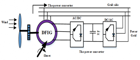
Figure 1. DFIG based wind turbine scheme
The diagram of the DFIG wind turbine connected to the grid, including the various mechanical and electrical quantities used to model the electromechanical conversion chain, is shown in Figure 1 [5].
2.1 Model of the wind
The characteristics of the wind will determine the amount of energy that can actually be extracted from the wind farm [6].
The wind speed will be modeled in deterministic form by a sum of several harmonics:
$V_{v}=8+0.2 \sin (0.1047 . t)+2 \sin (0.2665 . t)+0.2 \sin (3.6645 . t)$ (1)
Wind energy comes from the kinetic energy of the wind. Indeed, if we consider a mass of air, m, which moves with velocity v, the kinetic energy of this mass is given by:
$E_{c}=\frac{1}{2} m v^{2}$ (2)
If, during the unit of time, this energy could be completely recovered by means of a propeller that sweeps a surface S, located perpendicularly to the direction of the wind speed, the instantaneous power supplied would be, then:
$P_{v}=\frac{1}{2} \rho S v^{3}$ (3)
The Betz limit characterizes the ability of the wind turbine to capture wind energy. The corresponding power is given by [7]:
$P_{t}=C_{p}(\beta, \lambda) \frac{1}{2} \rho \pi R^{2} v^{3}$ (4)
The maximum power that can be collected by a wind turbine is calculated by the Betz limit:
$P_{t}^{\max }=C_{p}^{\max }(\beta, \lambda) \frac{1}{2} \rho \pi R^{2} v^{3}=0.593 P_{v}$ (5)
Thus, the notion of aerodynamic efficiency $\eta$ of the wind turbine can be defined by the ratio:
$\eta=\frac{C_{p}}{C_{p}^{\max }}=\frac{C_{p}}{0.539}$ (6)
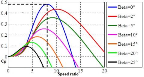
2.2 Power coefficient
The power coefficient $C_{p}$ depends on the number of blades of the rotor and their geometrical and aerodynamic shapes (length and profile of the sections). These are designed according to the characteristics of the site, the desired nominal power, the type of regulation (in pitch or stall) and the type of operation (fixed or variable speed) [8, 9].
Numerical approximations have been developed in the literature to model the coefficient $C_{p}$ and different expressions have been proposed [10, 11].
$\begin{align} & {{C}_{p}}(\beta ,\lambda )=(0.5-0.067(\beta -2))\sin [\frac{\pi (\lambda +0.1)}{18.5-0.3(\beta +2)} \\ & -0.00184(\lambda -3)(\beta -2)] \\\end{align}$ (7)
Figure 2. Coefficient of power of DFIG
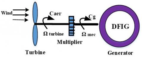
The multiplier adapts the speed (slow) of the turbine to the speed of the generator (Figure 3). This multiplier is modeled mathematically by the following equations [12]:
Figure 3. Diagram of the wind turbine
$C_{g}=\frac{c_{a e r}}{G}$ (8)
$\Omega_{\text {turbine}}=\frac{\Omega_{m e c}}{G}$ (9)
With: G: Gain of the speed multiplier.
The mass of the wind turbine is transferred to the turbine shaft in the form of an inertia $J_{turbine}$ and comprises the mass of the blades and the rotor mass of the turbine.
$J=\frac{J_{\text {turbine}}}{G^{2}}+J_{g}$ (10)
The fundamental equation of the dynamics makes it possible to determine the evolution of the mechanical speed from the total mechanical torque ($C_{m e c}$) applied to the rotor:
$J \frac{d \Omega_{m e c}}{d t}=C_{m e c}$ (11)
J: is the total inertia that appears on the rotor of the generator. This mechanical torque takes into account, the electromagnetic torque $\mathrm{C}_{\mathrm{em}}$ produced by the generator, the viscous friction couple $C_{f}$, and the torque $C_{g}$.
The mechanical torque applied to the rotor:
$J \frac{d \Omega_{m e c}}{d t}=C_{m e c}=C_{g}-C_{e m}-C_{f}$ (12)
The resistant torque due to friction is modeled by a coefficient of viscous friction f:
$C_{f}=f \Omega_{m e c}$ (13)
Figure 4. Power coefficient of DFIG
The DFIG has three stator equations and three rotor equations:
$\left\{\begin{array}{l}{\left[V_{s a b c}\right]=-\left[R_{s}\right]\left[I_{s a b c}\right]+\frac{d \varphi_{r a b c}}{d t}} \\ {\left[V_{r a b c}\right]=\left[R_{r}\right]\left[I_{r a b c}\right]+\frac{d \varphi_{s a b c}}{d t}}\end{array}\right.$ (14)
$\left\{\begin{array}{l}{\left[\varphi_{s a b c}\right]=-\left[L_{s s}\right]\left[I_{s a b c}\right]+\left[M_{s r}\right]\left[I_{s a b c}\right]} \\ {\left[\varphi_{r a b c}\right]=-\left[M_{s r}\right]\left[I_{r a b c}\right]+\left[L_{r r}\right]\left[I_{r a b c}\right]}\end{array}\right.$ (15)
The four-inductor matrices are:
$\left[L_{ss}\right]=\left[\begin{array}{ccc}{L_{s}} & {M_{s}} & {M_{s}} \\ {M_{s}} & {L_{s}} & {M_{s}} \\ {M_{s}} & {M_{s}} & {L_{s}}\end{array}\right] ;\left[L_{r r}\right]=\left[\begin{array}{ccc}{L_{r}} & {M_{r}} & {M_{r}} \\ {M_{r}} & {L_{r}} & {M_{r}} \\ {M_{r}} & {M_{r}} & {L_{r}}\end{array}\right]$ (16)
$L_{s}$ and $L_{r}$ are respectively the stator and rotor inductors.
$M_{s}$ and $M_{r}$ are respectively the mutual stator and rotor inductances.
$\left[M_{s r}\right]=\left[M_{r s}\right]^{T}=M\left[\begin{array}{ccc}{\cos \theta} & {\cos \left(\theta-\frac{4 \pi}{3}\right)} & {\cos (\theta-2 \pi / 3)} \\ {\cos (\theta-2 \pi / 3)} & {\cos \theta} & {\cos \left(\theta-\frac{4 \pi}{3}\right)} \\ {\cos \left(\theta-\frac{4 \pi}{3}\right)} & {\cos (\theta-2 \pi / 3)} & {\cos \theta}\end{array}\right]$ (17)
The dynamic equation is:
$J \frac{d \Omega}{d t}=C_{e m}-C_{r}-f \Omega$ (18)
Magnetic equations:
$\left\{\begin{array}{l}{\varphi_{d s}=L_{s} I_{d s}+M I_{d r}} \\ {\varphi_{q s}=L_{s} I_{q s}+M I_{q r}} \\ {\varphi_{d r}=L_{r} I_{d r}+M I_{d s}} \\ {\varphi_{q r}=L_{r} I_{q r}+M I_{q s}}\end{array}\right.$ (19)
Stator and rotor voltages:
$\left\{\begin{aligned} V_{d s} &=R_{s} I_{d s}+\frac{d \varphi_{d s}}{d t}-\omega_{s} \varphi_{q s} \\ V_{q s} &=R_{s} I_{q s}+\frac{d \varphi_{q s}}{d t}-\omega_{s} \varphi_{d s} \\ V_{d r} &=R_{r} I_{d r}+\frac{d \varphi_{d r}}{d t}-\left(\omega_{s}-\omega_{r}\right) \varphi_{q r} \\ V_{q r} &=R_{r} I_{q r}+\frac{d \varphi_{q r}}{d t}-\left(\omega_{s}-\omega_{r}\right) \varphi_{d r} \end{aligned}\right.$ (20)
Expression of active and reactive power:
$\left\{\begin{array}{l}{P_{s}=V_{d s} I_{d s}+V_{q s} I_{q s}} \\ {Q_{s}=V_{q s} I_{d s}-V_{d s} I_{q s}}\end{array}\right.$ (21)
$\left\{\begin{array}{l}{P_{r}=V_{d r} I_{d r}+V_{q r} I_{q r}} \\ {Q_{r}=V_{q r} I_{d r}-V_{d r} I_{q r}}\end{array}\right.$ (22)
The purpose of the vector control is to control the asynchronous machine as an independently excited DC machine where there is a natural decoupling between the magnitude controlling the flux (the excitation current) and that related to the torque (the armature current). This decoupling provides a very fast torque response, a large speed control range and high efficiency for a large steady state load range [13].
Examination of the expression of the torque of the machine shows that it results from a difference between two quadrature components of the stator current and rotor flux which has a complex coupling between the machine magnitudes. The working reference for the control is that related to the rotating field so that the axis (d) coincides with the direction desired flow, which can be rotor, stator, or air gap. Thus, it is possible to orient the different flows of the machine [14, 16].
The stator flux with the conditions:
$\left\{\begin{array}{c}{\varphi=\varphi_{d s}=\varphi_{s}} \\ {\varphi_{q s}=0}\end{array}\right.$ (23)
The rotor flow with the conditions:
$\left\{\begin{array}{c}{\varphi=\varphi_{d r}=\varphi_{r}} \\ {\varphi_{q r}=0}\end{array}\right.$ (24)
For a DFIG, the relation of the electromagnetic torque is given by the following equation:
$C_{e m}=\frac{3}{2} \frac{L_{m}}{L_{s}} p\left(\varphi_{q s} i_{d r}-\varphi_{d s} i_{q r}\right)$ (25)
Starting from Eq. (25), a decoupling can be performed in such a way that the torque will be controlled solely by the current
and thus the flow by the current . The final relationship of the couple is:$C_{e m}=-\frac{3}{2} \frac{L_{m}}{L_{s}} p\left(\varphi_{s} i_{q r}\right)$ (26)
$\left\{\begin{array}{c}{V_{d s}=0} \\ {V_{q s}=V_{s}=\omega_{s} \varphi_{s}}\end{array}\right.$ (27)
$\left\{\begin{array}{c}{\varphi_{s}=L_{s} I_{d s}+M I_{d r}} \\ {0=L_{s} I_{q s}+M I_{q r}}\end{array}\right.$ (28)
We get the following expressions for the active and reactive powers:
$\left\{\begin{array}{c}{P_{s}=-V \frac{L_{m}}{L_{s}} I_{q r}} \\ {Q_{s}=V_{s} \frac{\varphi_{s}}{L_{s}}-V_{s} \frac{L_{m}}{L_{s}} I_{d r}}\end{array}\right.$ (29)
By drawing: $\varphi_{s}=\frac{V_{s}}{\omega_{s}}$ from equation (27), the expression of the reactive power becomes:
$Q_{s}=\frac{V_{s}^{2}}{L_{s} \omega_{s}}-\frac{V_{s} L_{m}}{L_{s}} I_{d r}$ (30)
The expression of the powers (29) can thus be simplified in the following way:
$\left\{\begin{array}{c}{P=-V_{s} \frac{M}{L_{s}} i_{q r}} \\ {Q=-V_{s} \frac{M}{L_{s}} i_{d r}+\frac{V_{s}^{2}}{L_{s} \omega_{s}}}\end{array}\right.$ (31)
Direct Power Control (DPC) is based on the concept of direct torque control applied to electrical machines. The goal is to directly control active and reactive power in a PWM rectifier. The errors between the reference values of the instantaneous active and reactive powers and their measurements are introduced in two hysteresis comparators which determine the switching state of the semiconductors, with the help of a switchboard and the value of the sector where the voltage of the generator [17].
6.1 General principle of DPC
The overall structure of the DPC, using a predefined switching table, applied to the three-phase machine-side converter is shown in Figure 5. It is similar to that of the direct torque control (DTC). Instead of torque and rotor flux, it is the active and reactive stator power that is the controlled quantities.
The principle of the DPC consists in selecting a sequence of switching commands (Sa, Sb, Sc) of the semiconductors constituting, from a switching table. The selection is made on the basis of the errors (εPs and εQs) between the references of the active and reactive powers ($P_{S}^{*}$ and $Q_{S}^{*}$) and the real values(Ps and Qs), provided by two comparators to hysteresis of digitized outputs HP and HQ respectively, as well as on the sector (zone) in which the vector of the rotor flux is [18, 19].
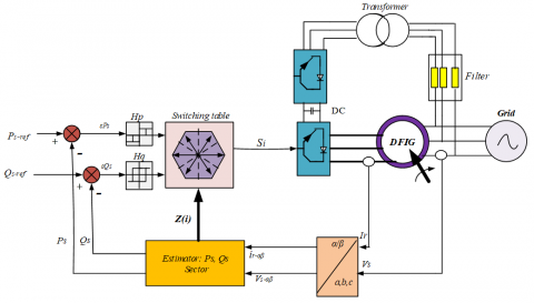
Figure 5. DPC configuration of the DFIG
In order to achieve a switching table providing simultaneous control of the active and reactive powers, in all sectors, it is essential to study the variations caused by the application of each of the control vectors on the latter, and this at the same time. During a complete period of rotor voltage. The control vectors selected in this switching table must ensure the restriction of the reference tracking error of the two active and reactive powers, simultaneously.
6.2 Estimation of active and reactive power
Instead of measuring the powers on the network, capturing the rotor currents, and estimate Ps and Qs. This approach gives early control of the powers in the stator windings. That is, the one established by neglecting the resistance of the stator phase. We can find the relations of Ps and Qs according to the two components of the rotor flux in the reference frame (αr-βr) [19, 20, 23].
The active and reactive powers are controlled by two hysteresis comparators, the measured values of the powers being estimated from the following relationships [21, 22]:
$\left\{ \begin{array} { c } { P _ { s } = - \frac { 3 } { 2 } \frac { L _ { m } } { \sigma L _ { s } L _ { r } } V _ { s } \varphi _ { r \beta } } \\ { Q _ { s } = \frac { 3 } { 2 } \left( \frac { V _ { s } } { \sigma L _ { s } } \varphi _ { s } - \frac { V _ { s } L _ { m } } { \sigma L _ { s } L _ { r } } \varphi _ { r \alpha } \right) } \end{array} \right.$ (32)
From where,
$\left\{ \begin{aligned} \varphi _ { r \alpha } = & \sigma L _ { r } i _ { r \alpha } + \frac { L _ { m } } { L _ { s } } \varphi _ { s } \\ \varphi _ { r \beta } & = \sigma L _ { r } i _ { r \beta } \\ | \overrightarrow { \varphi _ { s } } | & = \frac { | \overrightarrow { V _ { s } } | } { \omega _ { s } } \\ \sigma & = 1 - \frac { L _ { m } ^ { 2 } } { L _ { s } L _ { r } } \end{aligned} \right.$ (33)
If, by introducing the angle δ between the stator and rotor flux vector, Ps and Qs become:
$\left\{ \begin{array} { c } { P _ { s } = - \frac { 3 } { 2 } \frac { L _ { m } } { \sigma L _ { s } L _ { r } } \omega _ { s } \left| \varphi _ { s } \| \varphi _ { r } \right| \sin \delta } \\ { Q _ { s } = \frac { 3 } { 2 } \frac { \omega _ { s } } { \sigma L _ { s } } \left| \varphi _ { s } \right| \left( \frac { L _ { m } } { L _ { r } } \left| \varphi _ { r } \right| \cos \delta - \left| \varphi _ { s } \right| \right) } \end{array} \right.$ (34)
The derivative of the two equations in (34) gives:
$\left\{ \begin{aligned} \frac { d P _ { s } } { d t } = & - \frac { 3 } { 2 } \frac { L _ { m } } { \sigma L _ { s } L _ { r } } \omega _ { s } \left| \varphi _ { s } \right| \frac { d \left| \varphi _ { r } \right| \sin \delta } { d t } \\ \frac { d Q _ { s } } { d t } & = \frac { 3 } { 2 } \frac { L _ { m } \omega _ { s } } { \sigma L _ { s } L _ { r } } \left| \varphi _ { s } \right| \frac { d \left( \left| \varphi _ { r } \right| \cos \delta \right) } { d t } \end{aligned} \right.$ (35)
As can be seen in (23), these last two expressions show that the active and reactive stator powers can be controlled by the modification of the relative angle δ between the stator and rotor flux vectors and their amplitudes.
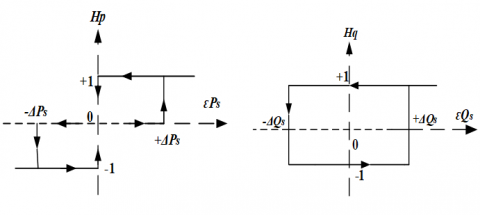
6.3 Choice of hysteresis comparators
In order to obtain very good dynamic performances, the choice of a two-level hysteresis corrector seems to be the simplest and best solution for controlling the active and reactive power. These comparators (Figure 6) must make it possible to control the exchange of the active and reactive power between the DFIG and the power grid in both directions and with the two modes of hypo and hyper-synchronous operation of the DFIG.
Figure 6. Hysteresis comparators: active power, reactive power
Similar to DTC, the DPC for DFIG is based on the selection of a rotor voltage vector such that errors between measured and reference quantities are reduced and maintained between the limits of the hysteresis bands.
6.4 Switching table
To select the optimum rotor voltage vector, it is necessary to know the relative position of the rotor flux in the six sextants. A three-phase inverter with two voltage levels can produce eight different combinations; these eight combinations generate eight voltage vectors that can be applied to the rotor terminals of the DFIG.
The division of the complex plane into six angular zones Zi(i = 1.....6) can be determined by the following relation:
$- \frac { \pi } { 6 } + ( i - 1 ) \frac { \pi } { 3 } \leq Z _ { i } < \frac { \pi } { 6 } + ( i - 1 ) \frac { \pi } { 3 }$ (36)
It follows that Table 2 of the optimal vectors is derived in the same way by giving priority to the control of the active power on the reactive power. The signals of Hp and HQ thus the rotor flux vector position δ, represent the inputs of this truth table, whereas the switching states $S _ { a } , S _ { b } , S _ { c }$ represent its output.
Table 1. Optimal vector selection table [21]
|
Rp |
1 |
-1 |
|||||
|
Rq |
1 |
0 |
-1 |
1 |
0 |
-1 |
|
|
Rotor flux sector |
1 |
V5 |
V7 |
V3 |
V6 |
V0 |
V2 |
|
2 |
V6 |
V0 |
V4 |
V1 |
V7 |
V3 |
|
|
3 |
V1 |
V7 |
V5 |
V2 |
V0 |
V4 |
|
|
4 |
V2 |
V0 |
V6 |
V3 |
V7 |
V5 |
|
|
5 |
V3 |
V7 |
V1 |
V4 |
V0 |
V6 |
|
|
6 |
V4 |
V0 |
V2 |
V5 |
V7 |
V1 |
|
Nevertheless, the fundamental reality on which the DPC is based is that the movement of the rotor flux in the machine follows a continuous progression in time and that it will seem to cross each sector one by one if it is sampled sufficiently. The study in Table 2 indicates that if the rotor flux was for example in sector 2 and the vector V3 had just been applied, the variation of the reactive power measured at the stator must inevitably be negative since the vector V3 decreases the reactive power to the stator. If this had not been the case, we would have to admit that our estimate of the sector is no longer fair and that the flow would rather be in sector 1 or 5. Table 3 presents the signs of the variations of the instantaneous active and reactive powers for each input voltage vector of the rectifier according to the sector where the voltage of the generator is located. By choosing the appropriate output vector, it is possible to select the signs of variation of the active and reactive powers independently.
Table 2. DFIG parameters
|
Parameter name |
Symbol |
Value |
Unit |
|
Rated power |
Pn |
1.5 |
MW |
|
Rated current |
In |
1900 |
A |
|
Rated DC-Link voltage |
UDC |
1200 |
V |
|
Stator rated voltage |
Vs |
398/690 |
V |
|
Stator rated frequency |
f |
50 |
Hz |
|
Rotor inductance |
Lr |
0.0136 |
H |
|
Stator inductance |
Ls |
0.0137 |
H |
|
Mutual inductance |
M |
0.0135 |
H |
|
Rotor resistance |
Rr |
0.021 |
Ω |
|
Stator resistance |
Rs |
0.012 |
Ω |
|
Number of pair of poles |
p |
2 |
- |
Table 3. Wind turbine parameters
|
Parameter name |
Symbol |
Value |
Unit |
|
The power coefficient |
Cpmax |
0.48 |
- |
|
Rotor radius |
R |
35.25 |
m |
|
Speed multiplier gain |
G |
90 |
- |
|
The density of the air |
ρ |
1.225 |
kg/m3 |
|
Moment of total inertia |
J |
1000 |
Kg.m2 |
|
Viscous friction coefficient |
fr |
0.0024 |
N.m.s-1 |
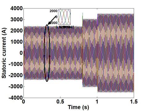
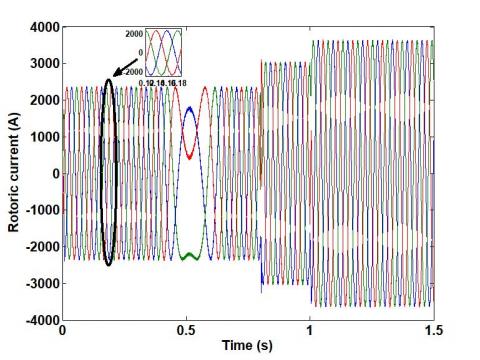
The stator current generated by the DFIG which has a sinusoidal shape (Figure 7 and Figure 8), which means a good quality of energy supply to the power grid.
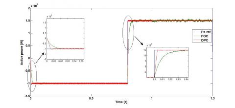
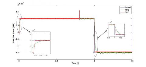
From the results of the simulation obtained in Figure.9 and Figure.10, we can say that the control DPC response time is very fast compared to the FOC control with high performance (tracking instructions, very fast response time, no overshoot, minimal static error).
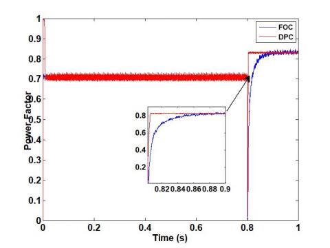
According to Figure 11, the power factor obtained by the two control strategies is variable according to the values of the active and reactive powers. To keep a unit power factor on the network side, the stator reactive power set point will be kept zero (Qs-ref = 0MVAR), this is the objective of the next test.
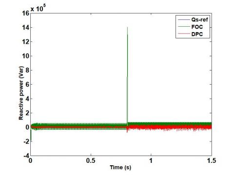
Figure 12 illustrates the reactive power injected into the array by the assembly. We set ourselves a zero instruction to have a unity power factor on the network side.
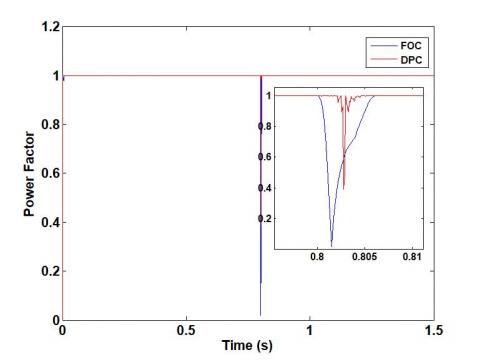
Figure 13 shows that the unit power factor (PF) more stable for DPC versus FOC.
Figure 7. Stator currents (DPC)
Figure 8. Rotor currents (DPC)
Figure 9. Active power (FOC, DPC)
Figure 10. Reactive power (FOC, DPC)
Figure 11. Power factor of DFIG (FOC, DPC)
Figure 12. Reactive power (FOC, DPC)
Figure 13. Power Factor of DFIG (FOC, DPC)
This paper has been dedicated to the modelling, simulation and analysis of a wind turbine operating at variable speed. The DPC technique is applied for the tow side (grid and rotor side). The proposed scheme has the advantages of simple algorithm, good dynamic performances, good quality of energy supplied to the electricity network. Advantages of the DPC control structure of very high dynamic response, no use of nested loops, coordinate or modulator transformations, or decoupling of current components. Based on the obtained results, it can be concluded that the robust control method can be a very attractive solution for devices using DFIG, such as wind energy conversion systems.
AC Alternating Current
DC Direct Current
PF Power Factor
Cp Power coefficient
R Blade radius (m)
Rs, Rr Stator and rotor resistances (Ω)
Ls, Lr Self inductance of stator and rotor (H)
M Mutual magnetizing inductance
φs, φr Stator and rotor flux (Wb)
Cem Electromagnetic torque (Nm)
v Wind speed (m/s)
J Inertia moment of the moving element (kgm2)
λ Ratio of speed
ρ Air density
β Pitch angle
fr Viscous friction coefficient
p Number of pair poles
G Mechanical speed multiplier
ωs Synchronously rotating angular speed (rad/s)
ωr Electrical angular rotor speed (rad/s)
Vs, Vr Stator and rotor voltage (V)
Idr, Iqr Direct and quadrature component of the rotor currents (A)
Ids, Iqs Direct and quadrature component of the stator currents (A)
g Slip
Ω Mechanical speed (rad/s)
P Active power (W)
Q Reactive power (Var)
[1] Noguchi, T., Tomiki, H., Kondo, S., Takahashi, I. (1996). Direct power control of PWM converter without power source voltage sensors. In IAS ’96. Conference Record of the 1996 IEEE Industry Applications Conference Thirty-First IAS Annual Meeting, 2: 941-946. https://doi.org/10.1109/IAS.1996.560196
[2] Çadirci, I., Ermiş, M. (1992). Double-output induction generator operating at subsynchronous and supersynchronous speeds: Steady-state performance optimisation and wind-energy recovery. IEE Proceedings B (Electric Power Applications), 139(5): 429-442. https://doi.org/10.1049/ip-b.1992.0053
[3] Shehata, E.G. (2015). Sliding mode direct power control of RSC for DFIGs driven by variable speed wind turbines. Alexandria Engineering Journal, 54(4): 1067-1075. https://doi.org/10.1016/J.AEJ.2015.06.006
[4] Bossanyi, E., Burton, T., Sharpe, D., Jenkins, N. (2000). Wind Energy Handbook. New York: Wiley. http://library.uniteddiversity.coop/Energy/Wind/Wind_Energy_Handbook.pdf
[5] Kahla, S., Soufi, Y., Sedraoui, M., Bechouat, M. (2015). On-Off control based particle swarm optimization for maximum power point tracking of wind turbine equipped by DFIG connected to the grid with energy storage. International Journal of Hydrogen Energy, 40(39): 13749-13758. https://doi.org/10.1016/J.IJHYDENE.2015.05.007
[6] Amrane, F., Chaiba, A. (2015). A hybrid intelligent control based on DPC for grid-connected DFIG with a fixed switching frequency using MPPT strategy. In: 4th International Conference on Electrical Engineering (ICEE), Boumerdes, Algeria, pp. 1-4. https://doi.org/10.1109/INTEE.2015.7416678
[7] Şeker, M., Zergeroğlu, E., Tatlicioğlu, E. (2016). Non-linear control of variable-speed wind turbines with permanent magnet synchronous generators: A robust backstepping approach. International Journal of Systems Science, 47(2): 420-432. https://doi.org/10.1080/00207721.2013.834087
[8] Çadirci, I., Ermiş, M. (1992). Double-output induction generator operating at subsynchronous and supersynchronous speeds: steady-state performance optimisation and wind-energy recovery. IEE Proceedings B (Electric Power Applications), 139(5): 429-442. https://doi.org/10.1049/ip-b.1992.0053
[9] Aboulem, S., Boufounas, E.M., Boumhidi, I. (2017) Optimal tracking and robust intelligent based PI power controller of the wind turbine systems. Intelligent Systems and Computer Vision, Fez, Morocco. https://doi.org/10.1109/ISACV.2017.8054981
[10] Barambones, O. (2019). Robust wind speed estimation and control of variable speed wind turbines. Asian Journal of Control, 21(2): 856-867. https://doi.org/10.1002/asjc.1779
[11] Poitiers, F., Bouaouiche, T., Machmoum, M. (2009). Advanced control of a doubly-fed induction generator for wind energy conversion. Electr Power Syst Res, 79(7): 1085-1096. https://doi.org/10.1016/J.EPSR.2009.01.007
[12] Boyette, A. (2006). Contrôle-commande d’un générateur asynchrone à double alimentation avec système de stockage pour la production éolienne. Université Henri Poincaré - Nancy 1.
[13] Sawada, M., Itamiya, K. (2011). A design scheme of model reference adaptive control system with using a smooth parameter projection adaptive law. In SICE Annual Conference 2011, pp. 1704-1709. https://ieeexplore.ieee.org/abstract/document/6060241
[14] Rudraraju, V.R.R., Nagamani, C., Ilango, GS. (2015). A control scheme for improving the efficiency of DFIG at low wind speeds with fractional rated converters. Int J Electr Power Energy Syst, 70: 61-9. https://doi.org/10.1016/J.IJEPES.2015.01.032
[15] Ko, H.S., Yoon, G.G., Kyung, N.H., Hong, W.P. (2008). Modeling and control of DFIG-based variable-speed wind-turbine. Electr Power Syst Res, 78(11): 1841-1849. https://doi.org/10.1016/J.EPSR.2008.02.018
[16] Mouilah, K., Abid, M., Naceri, A., Allam, M. (2014). Fuzzy Control of a Doubly Fed Induction Generator for Wind Turbines’. J. Electr. Eng. JEE, 14(4): 352-357.
[17] Abosh, A.H., Zhu, Z.Q., Ren, Y. (2017). Reduction of torque and flux ripples in space vector modulation-based direct torque control of asymmetric permanent magnet synchronous machine. IEEE Transactions on Power Electronics, 32(4): 2976-2986. https://doi.org/10.1109/TPEL.2016.2581026
[18] Antoniewicz, P., Kazmierkowski, M.P. (2008). Virtual-flux-based predictive direct power control of AC/DC converters with online inductance estimation. IEEE Trans. Ind. Electron., 55(12): 4381-4390. https://doi.org/10.1109/TIE.2008.2007519
[19] Bektache, A., Boukhezzar, B. (2018). Nonlinear predictive control of a DFIG-based wind turbine for power capture optimization. Int J Electr Power Energy Syst, 101: 92-102. https://doi.org/10.1016/J.IJEPES.2018.03.012
[20] Datta, R., Ranganathan, V.T. (2001). Direct power control of grid-connected wound rotor induction machine without rotor position sensors. IEEE Trans. Power Electron., 16(3): 390-399. https://doi.org/10.1109/63.923772
[21] Abad, G., Rodriguez, M.A., Poza, J. (2007). Predictive direct power control of the doubly fed induction machine with reduced power ripple at low constant switching frequency. In 2007 IEEE International Symposium on Industrial Electronics, pp. 1119-1124. https://doi.org/10.1109/ISIE.2007.4374755
[22] Bouyekni, A., Taleb, R., Boudjema, Z., Kahal, H. (2018). A second-order continuous sliding mode based on DPC for wind-turbine-driven DFIG. Elektroteh Vestn, 85: 29-36.
[23] Shehata, E.G. (2015). Sliding mode direct power control of RSC for DFIGs driven by variable speed wind turbines. Alexandria Eng J., 54: 1067-75. http://doi.org/10.1016/j.aej.2015.06.006