Ling Chen* | Wei Han | Yuhui Huang | Xiang Cao | Zikun Xu
OPEN ACCESS
Partial shading suppresses the output voltage and current of photovoltaic (PV) array, reduces the array efficiency and even causes the hot spot effect. To alleviate these negative effects, this paper proposes a new model of partially shaded PV arrays with different structures, and explores the effects of shading on the output features. On this basis, the PV array was reconfigured to weaken the shading effects. In addition, the fruit fly optimization algorithm (FOA) was improved to track the maximum power points (MPPs) of the reconfigured PV array. The improved FOA and reconfigured PV array were proved valid through simulations. The research results shed new light on the optimization of PV power generation under partial shading.
partial shading, photovoltaic (PV) array, reconfiguration, fruit fly optimization algorithm (FOA)
Each photovoltaic (PV) unit outputs a small voltage and power. Hence, multiple PV units are often connected in series or parallel, forming a PV array. However, the PV array must operate in an environment without being shaded by trees, buildings or clouds. Otherwise, the array will face problems like output decline, the hot spot effect, and the failure of maximum power point tracking (MPPT). As a result, how to weaken the impacts of shadows on PV array has become a research hotspot.
The installation condition and shadow effects must be considered to ensure the efficiency of PV power generation. Walker et al. [1, 2] put forward a simulation model of PV panel according to the effects of temperature and irradiance on cell output, without considering the impacts of shadows. Picault and Raison [3, 4] explored the influencing of shadow on individual PV panel, but ignored the output features of large PV farm under shadows. Nguyen et al. [5-7] analyzed the output features of PV units under various shadow conditions, yet failing to model the complex PV generation conditions under shadows. Noguchi et al. [8-10] recommended models of PV modules under nonuniform irradiance, but did not discuss the PV size or pattern. Zhang et al. [11, 12] installed bypass diodes to provide low-impedance energy pathways to the shaded module. However, the bypass diodes lead to multiple local maximum power points (MPPs), calling for more sophisticated MPPT techniques. Karatepe et al. [13-15] designed a PV array that uses switches to adapt to different irradiances. The problem is that the designed array requires too many switches and supports only a few structural forms.
Starting from the structure of PV array, this paper explores the output features of PV array under shadows, and reconfigured the PV model to weaken the effect of partial shading. Next, the fruit fly optimization algorithm (FOA) was improved to track the MPPs, and optimize the output performance of the reconfigured PV structure under partial shading.
2.1 PV array model
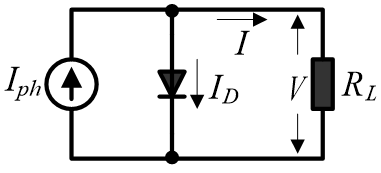
According to the principle of PV power generation, each PV unit is equivalent to thin p-n junction parallel with a diode. For example, Bian et al. [16, 17] considered each PV unit as a parallel structure of a diode and a current source, which converts solar energy into a light current. If the irradiance remains constant, the light current will not change with working conditions. In the equivalent circuit (Figure 1) of an ideal PV unit, there is a current source Iph that outputs a constant light current according to the irradiance. The light current partially flows through the load RL to form the load voltage V. Meanwhile, the voltage acts as a positive bias on the p-n junction diode, creating a dark current ID opposite to the light current.
Figure 1. Equivalent circuit of an ideal PV unit
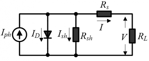
In practice, the equivalent circuit of each PV unit also contains a series resistor Rs and a parallel resistor Rsh, the capacitance of p-n junction, and distributed capacitance. The capacitances can be ignored in the equivalent circuits, because the PV unit is a direct-current (DC) device with no high-frequent components. Figure 2 shows the equivalent circuit of a practical PV unit.
Figure 2. Equivalent circuit of a practical PV unit
2.2 Mathematical model of PV array
According to the equivalent circuit and Kichhoff’s circuit laws, the currents in the PV array can be described as:
$I=I_{p h}-I_{D}-I_{S h}$ (1)
$I_{p h}=I_{s c}\left(\frac{s}{1000}\right)+C_{T}\left(T-T_{r e f}\right)$ (2)
$I_{D}=I_{0}\left[\exp \left(\frac{q V}{n k T}\right)-1\right]$ (3)
$I_{0}=I_{d 0}\left(\frac{T}{T_{r e f}}\right)^{3} \exp \left[\frac{q E_{g}}{n k}\left(\frac{1}{T_{r e f}}-\frac{1}{T}\right)\right]$ (4)
$I_{s h}=\frac{V+I R_{S}}{R_{s h}}$ (5)
where, I is the output current of the load; Iph is the light current affected by irradiance and temperature; ID is the diode current; Ish the current passing through the parallel resistor; Id0 is the reverse saturation current; Isc is the short-circuit current; q is the electron charge (constant); S is the irradiance; n is the diode emission coefficient; CT is the temperature coefficient; k is the Boltzmann constant; T is the temperature; Tref is the reference temperature; Eg is the band gap energy of silicon semiconductor (1.1~1.2eV).
In a PV array, the parallel resistance Rsh is usually assumed as infinitely large, due to its negligible impact on the output power. By contrast, the value and variation of series resistance Rs cannot be ignored, because of its significant impacts on output power. If the output current of the load I=0, then the voltage is open-circuit voltage Voc. By formulas (1) and (3), the open-circuit voltage Voc, the output current, and the output power can be obtained as:
$V_{O C}=\frac{n k T}{q} \ln \left(\frac{I_{p h}}{I_{0}}+1\right)$ (6)
$I=I_{p h}-I_{D}-\frac{V+I R_{S}}{R_{S h}} \approx I_{p h}-I_{D}=I_{p h}-I_{0}\left[\exp \left(\frac{q V}{n k T}\right)-1\right]$ (7)
$P=V I=V I_{p h}-V I_{0}\left[\exp \left(\frac{q V}{n k T}\right)-1\right]$ (8)
Each PV array is made up of units arranged in parallel or in series patterns. The serial units can increase the output of DC voltage, and the parallel units can boost the output of DC current. The number of units in each pattern determines the level of output current and power. Let ns be the number of serial units and np be the number of parallel units. By formulas (7) and (8), the output current and the output power of a PV array can be obtained as:
$I=n_{p} I_{p h}-n_{p} I_{0}\left[\exp \left(\frac{q}{n k T} \frac{V}{n_{s}}\right)-1\right]$ (9)
$P=V I=n_{p} V I_{p h}-n_{p} V I_{0}\left[\exp \left(\frac{q}{n k T} \frac{V}{n_{S}}\right)-1\right]$ (10)
Figure 3. Power-voltage curves of a PV array
Based on formula (10), the power-voltage curves of a PV array were plotted under different temperatures or irradiances. As shown in Figure 3, the short-circuit current is directly proportional to irradiation, and less related to temperature; the open-circuit voltage is significantly negatively correlated with temperature; the maximum output power increased with irradiance and decreased with temperature (creating a unique MPP). To sum up, the output power of the PV array is positively correlated with temperature and negatively with irradiance. The actual output power is the interactive results between temperature and irradiance.
3.1 Modelling of PV array under partial shading
Partial shading is common to PV arrays in actual operations. This phenomenon may be caused by objects like trees, buildings and clouds, and may also arise from defects and cracks on the array. There is a huge gap between the PV arrays with or without partial shading in maximum output power. The position of the shadow directly affects the model and output of PV array. Therefore, the partial shading must be fully explored to increase the output power of PV array.
In this section, the PV array under partial shading is modelled in reference to previous research. For example, Raushenbach [18] simulated the reverse avalanche breakdown of PV with double diode circuit model, established a mathematical model of shadows under constant temperature, and analyzed the current-voltage and power-voltage curves of PV arrays under partial shading. Chao et al. [19, 20] explored the features of PV array with serial units under partial shading.
Under partial shading, the shading ratio α was introduced to describe the percentage of irradiance blocked by the shadow. If α=0.1, then 10% of irradiance is blocked and (1-α) of irradiance is transmitted. Then, the light current generated under partial shading can be illustrated as:
$I_{p h}=\frac{(1-\alpha) S}{1000} I_{p h 0}$ (11)
where, Iph0 is the light current under standard test condition (STC); α can be defined as:
$\alpha=1-\frac{S_{b e h i n d}}{S}$ (12)
where, S is the irradiance before the shadow; Sbehind is the irradiance after the shadow.
3.1.1 Modelling of PV array under partial shading with constant temperature
(1) Modelling of PV array with parallel units under partial shading
The circuit of PV array with parallel units is displayed in Figure 4, where V1 and I1 are terminal voltage and current of PV1, respectively; V2 and I2 are terminal voltage and current of PV2, respectively.
Figure 4. The circuit of PV array with parallel units
It is assumed that PV1 is not shaded, while PV2 is shaded with the shading ratio α. Then, the light current of the PV array can be described as:
$I=I_{1}+I_{2}=\frac{(2-\alpha) S}{1000} I_{p h 0}-2 I_{0}\left[\exp \left(\frac{q V}{n k T}\right)-1\right]$ (13)
(2) Modelling of PV array with serial units under partial shading
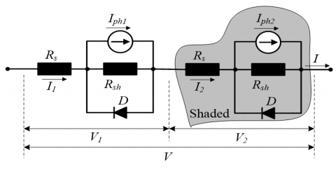
The circuit of PV array with serial units is displayed in Figure 5, where V1 and I1 are terminal voltage and current of PV1, respectively; V2 and I2 are terminal voltage and current of PV2, respectively.
Figure 5. The circuit of PV array with serial units
It is assumed that PV1 is not shaded, while PV2 is shaded with the shading ratio α. Then, the light current of the PV array can be described as:
$I=I_{p h 1}-\frac{\alpha S}{1000} I_{p h 0}-I_{0}\left[\exp \left(q \frac{V-\frac{n k T}{q} \ln \left(\frac{I_{p h 1}-I+I_{0}}{I_{0}}\right)}{n k T}\right)-1\right]$ (14)
Formula (14) shows the output current of the PV array is highly nonlinear with the changing irradiance, if the temperature remains constant.
3.1.2 Modelling of PV array under partial shading with constant irradiance
The temperature of the PV array varies with the irradiances, causing changes to the output features. The two factors basically have a linear relationship [21]. The temperature of the PV array can be estimated as:
$T=T_{a i r}+\frac{N O C T-20}{800} S$ (15)
where, NOCT is rated temperature of the PV array; Tair is the air temperature. The rated temperature is constant on the surface of the PV array. Here, the NOCT value is set to 48℃ according to the non-shaded irradiance (800W/m2) and air temperature (20℃).
(1) Modelling of PV array with parallel units under partial shading
According to the circuit diagram in Figure 4, the output currents of the two parallel PVs can be computed by:
$I_{1}=\frac{S}{1000} I_{p h 0}-I_{0}\left[\exp \left(\frac{q V_{1}}{n k\left(T_{a i r}+0.035 S\right)}\right)-1\right]$ (16)
$I_{2}=\frac{(1-\alpha) S}{1000} I_{p h 0}-I_{0}\left[\exp \left(\frac{q V_{2}}{n k\left(T_{\text {air }}+0.035(1-\alpha) S\right)}\right)-1\right]$ (17)
Then, the output current of the PV array can be obtained as:
$V=V_{1}=V_{2}$ (18)
$\begin{aligned} I=I_{1}+& I_{2}=\frac{(2-\alpha) S}{1000} I_{p h 0}-I_{0} \exp \left(\frac{q V}{n k\left(T_{\text {air}}+0.035 S\right)}\right) \\ &-I_{0} \exp \left(\frac{q V}{n k\left(T_{\text {air}}+0.035(1-\alpha) S\right)}\right)+2 I_{0} \end{aligned}$ (19)
(2) Modelling of PV array with serial units under partial shading
According to the circuit diagram in Figure 5, the output current of the PV array with serial units under partial shading can be described as:
$I=\frac{(1-\alpha) S}{1000} I_{p h 0}$$-I_{0}\left[\exp \left(\frac{q\left(V-\frac{n k\left(T_{a i r}+0.035 S\right)}{q} \ln \left(\frac{\frac{I p h_{0} S}{1000}-I+I_{0}}{I_{0}}\right)\right)}{n k\left(T_{a i r}+0.035(1-\alpha) S\right)}\right)-1\right]$ (20)
From formulas (19) and (20), it can be seen that the output current of the PV array is highly nonlinear with the changing temperature, if the irradiance remains the same.
3.2 Role of the diode
In the series circuit, a shaded PV unit will become a load that consumes the power generated by the other units. In this case, the temperature of the shaded unit will increase. The resulting hot spot effect will seriously damage the PV array.
To prevent the hot spot effect, a solution is to install a bypass diode beside the shaded unit. In normal cases, the PV unit will generate power with the diode in reverse bias. Once shaded, the PV unit will have a high resistance. The reverse bias of the unit will increase, making the diode conductive. Then, the current originally passing through the shaded unit will flow across the diode, such that the array can continue to produce electricity despite the shading effect. The flow diagram of the current with bypass diode is illustrated in Figure 6 below.
Besides preventing the hot spot effect, the installation of bypass diode also greatly enhances the output capacity of the array. The more the number of bypass diodes, the smaller the effect of partial shading on the PV array. In this research, the single-diode model is selected for equivalent circuit modelling.
Figure 6. Flow diagram of current with bypass diode
4.1 Structures of PV arrays
There are two basic structures of PV arrays: parallel and serial (Figures 4 and 5). The other structures are derived from the two basic ones. Figure 7 shows four common layouts of PV arrays, including the serial structure, the parallel structure, the asymmetric structure and the total-cross-tied (TCT) structure. The asymmetric structure is rarely used for PV arrays under uniform illumination. The TCT structure combines two series-parallel connections and a line AB.
Figure 7. Common layouts of PV arrays
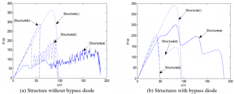
The serial, parallel and TCT structures output the same maximum power under uniform irradiance. Under partial shading, however, the three structure differ in the MPP. In this section, the PV arrays of serial, parallel, asymmetric and TCT structures are simulated under different shading conditions (GPV1=1,000W/m2, GPV2=800W/m2, GPV3=400W/m2 and GPV4=200W/m2), using the STC parameters provided by Suntech Power: Pm=170W, Voc=50V, Isc=4A, Vm=45V and Im=3.7A. To disclose the effects of diode on PV output, the PV arrays of the four structures were installed bypass diode, and simulated under the same shading conditions and STC parameters. The output power-voltage curves of the four structures, with or without bypass diode, are displayed in Figure 8 below.
Figure 8. Output power-voltage curves of the four structures under partial shading
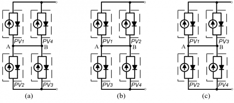
Figure 9. Three effective TCT structures
Figure 10. Output power-voltage curves of the three effective TCT structures
Next, the four PV units of the TCT structure were swapped, creating three effective structures (Figure 9) under nonuniform irradiance between the two series-parallel connections.
Then, the three effective TCT structures were simulated under different irradiances (GPV1=1000W/m2, GPV2=700W/m2, GPV3=500W/m2 and GPV4=200W/m2), with or without bypass diode. The output power-voltage curves thus obtained are displayed in Figure 10. Obviously, the different TCT structures had a gap of almost 100W in output power; structure (a) achieved the maximum output power, whether with or without bypass diode. Since the combined irradiance of G(PV1+PV4) equals that of G(PV2+PV3), there must be no shading between unit G(PV1+PV4) and unit G(PV2+PV3). This demonstrates an advantage of the TCT structure: the PV units have an equivalent balance that eliminates the shading effect on the PV array, without affecting the equal irradiance of each PV unit. Thus, the output power could be maximized by optimizing the structure of PV array under partial shading.
4.2 Reconfiguration of PV array
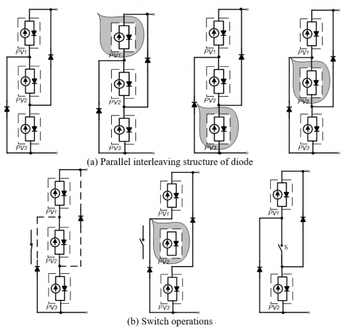
To control the number of diodes, the parallel interleaving structure was adopted to reduce the shading effect (Figure 11(a)). When the irradiance is completely uniform, the three PV units output current in series. When the bypass diode is reversed, PV2 can be regarded as a turn-on switch, while PV1 and PV3 as a series structure. If PV1 is fully shaded, PV3 will become a single circuit. If PV2 is fully shaded, the bypass diode will be conductive, and PV2 can be regarded as a turn-on switch, while PV1 and PV3 as a parallel structure. If PV3 is fully shaded, PV1 will become a single circuit.
The three different TCT structures were combined into a new structure of PV array (Figure 11(b)). In the new structure, the switch S and diode work together to turn PV1 and PV2 into series or parallel connections. When the switch S is open, the diode is under forward voltage, and the two PV units are parallel to each other, whichever the irradiance. In this case, the diode serves as a blocking diode. When the switch S is closed, the diode is in reverse bias, and the two PV units are under similar irradiance. Although the two units form a serial structure, the diode connected to the PV unit with weaker irradiance can transfer current. In this case, the diode is equivalent to a bypass diode in parallel connection, which protects the PV array against shading.
Figure 11. Circuit diagram of the new structure with switch and diode
Figure 12. Circuit diagram of the reconfigured PV array
Figure 12 shows the circuit of the reconfigured four-unit PV array. The four PV units are denoted as PV1, PV2, PV3 and PV4, respectively. On this basis, more structures can be designed with a few switches under partial shading.
Under partial shading, the traditional MPPT technique cannot track the local maximum of multiple outputs. Then, the output power of the PV array will decrease sharply. What is worse, the DC converter could not work normally under the reduced output voltage, and the entire array will operate in an inefficient manner. To overcome the defects, the FOA was improved and applied to the MPPT, with the aim to enhance MPPT performance and eliminate the effect of partial shading.
5.1 Global search of FOA
Inspired by the foraging behavior of fruit flies, the FOA provides a simple, fast and stable method [22] to search for the global optimal solution. The foraging strategy of fruit flies is illustrated in Figure 13. The fruit flies are known for their excellent visual and acoustic abilities. For example, a fruit fly can “smell” foods 40km away. When a fruit fly gets close to the food source, it will transmit information to the rest of the swarm and direct the flocking location of the swarm closer to the location of the food. Through iterative evolution, the fly swarm comes closer and closer to the food source, until the target is reached.
Figure 13. The foraging behavior of fruit flies
The FOA can be implemented in the following steps:
Step 1. Randomly initialize the position of each fruit fly in the swarm:
Init X_axis; Init Y_axis
Step 2. Set the random sensing direction and distance of each fruit fly:
Xi=X_axis+RandomValue; Yi=Y_axis+RandomValue
Step 3. Estimate the distance to origin (Dist), and compute the odor intensity judgement value (S), which is the reciprocal of distance: Dist$_{i}=\sqrt{X_{i}^{2}+Y_{i}^{2}} ; S_{i}=\frac{1}{\text { Dist }_{i}}$
Step 4. Substitute the S value into the odor intensity judgement function (fitness function), and find the odor intensity (Smelli) at the current position of the fruit fly:
Smelli=Function(Si)
Step 5. Find the fruit fly with the most intense odor in the swarm:
[bestSmell bestIndex]=max(Smell)
Step 6. Keep the highest odor intensity and the corresponding position (x, y). Then, the swarm will flock towards this position:
Smellbest=bestSmell
X_axis=X(bestindex)
Y_axis=Y(bestIndex)
Step 7. Repeat Steps 2-5, and, in each iteration, judge if the odor intensity is greater than that in the previous iteration. If yes, execute Step 6.
Compared with popular optimization algorithms (e.g. particle swarm optimization (PSO)), the FOA can track the global optimal solution with a low computing load, without falling into the local optimum trap.
5.2 Improved FOA
Considering the features and safety of PV array, the PV array structure should be optimized to maximize the output power. Then, the objective of PV array reconfiguration is to maximize the total output power:
$P \sum_{i=1}^{n} P V_{i \max }$ (21)
where, i=1, 2, 3 and 4 is the serial number of PV units. Different PV array structures may output the same power, and will produce different currents. Since the current depends on the PV unit stability, the energy of PV array should be managed by the following strategy: the output current should be reduced after the output power meets the set value, without sacrificing the output stability. It is known that the serial PV units increases open-circuit voltage, while parallel PV units increases short-circuit current; in addition, the parallel structure has a low output voltage and high current through DC bus, and thus a high power loss. Hence, the number of parallel circuits should be minimized to reduce the output current.
According to the above strategy and the independence of PV units, the PV array reconfiguration should satisfy two constraints:
$P \geq(1-\beta) P_{\max }$ (22)
$I \leq(1-2 \beta) I_{\max }$ (23)
where, P is the actual output power in the MPP; I is the actual output current in the MPP; b is the safety margin constraint.
For MPPT of PV array, the FOA mainly executes two tasks: search for global optimal solution and the MPPT. Each optimization problem of potential solution, i.e. the MPPT, was regarded as a fruit fly in the search space. Each fruit fly constantly decides its current fitness value. Taking the total output power of PV array as the target, the FOA-based MPPT was implemented in the following steps (Figure 14):
Figure 14. The flow chart of global search of the FOA
Step 1. FOA initialization
Initialize the position of each fruit fly in the swarm, the number of iterations, etc.
Step 2. Swarm evaluation
Compute the fitness value of each fruit fly. The objective function of the total output power of PV array can be expressed as:
$Smell_{i,j}=\sum_{j=1}^{m}\left[U_{j} \times \sum_{i=1}^{n} P V f u n\left(U_{j}, S u n_{i}, T_{i}\right)\right]$ (24)
where, PVfun is the output feature function of PV units at 25 ℃. The fitness value contains current and voltage, which can be adds up to form the output power.
Step 3. Fitness comparison and position update
Compare the current fitness of each fruit fly with the best-known fitness, and retain the larger one. After comparing the two values of all fruit flies, find the greatest fitness in the swarm. Then, update the position of each fruit fly according to the global optimal fitness.
Step 4. Termination
If the termination condition is satisfied, terminate the computation, and output the range of the optimal solution. Otherwise, return to Step 2 and repeat the above steps until reaching the maximum number of iterations.
To speed up convergence and avoid the local optimum trap, the FOA was improved by dividing the swarm into two parts. In one part, the fruit flies search for a better solution in a small range near the optimal solution. In the other part, the fruit flies search in a large range to avoid the local optimum trap.
5.3 MPPT of PV array
A PV array structure to be reconfigured were initially placed under a uniform irradiance of 1,000W/m2. Then, the irradiance started to vary under partial shading, such as GPV1=GPV3=1,000W/m2 and GPV2= GPV4=600W/m2. The output power-voltage curve of the original structure and reconfigured structure are shown in Figure 15(a). The maximum output power quickly declined from 605 to 260W (from point A to point B) with the change in irradiance, but rebound from 260 to 440W (from point B to point C) after the reconfiguration. Through the reconfiguration, the maximum output power saw a net increase of 180W.
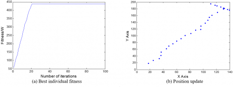
Both the FOA and the conventional incremental conductance (InC) algorithm were applied for MPPT. The results in Figure 15(b) show that the InC mistook the local maximum point D of the multi-peak curve as the optimal solution, resulting in power loss. By contrast, the improved FOA tracked the MPP accurately in fewer iterations, without falling into the local optimum trap. The optimization process of the FOA is explained in Figure 16.
Figure 15. Simulation results
Figure 16. The optimization process of improved FOA
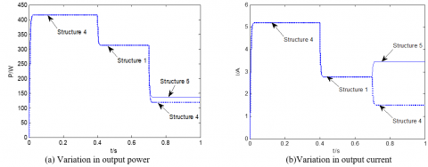
Figure 17. Structure selection under different irradiances
The reconfigured PV array also enjoys high reliability. Whenever one PV unit is damaged, the other PV units will work normally. During the simulation, the four PV units were arranged in series pattern, and the optimal structure was identified under the irradiances under varied shading conditions. The shading ratio b was set to 20%. Then, at t=0s, the irradiances were GPV1=1000W/m2, GPV2=800W/m2, GPV3=600W/m2 and GPV4=400W/m2, respectively; at t=0.4s, the irradiances were GPV1=600W/m2, GPV2=600W/m2, GPV3=100W/m2 and GPV4=600W/m2, respectively; at t=0.7s, the irradiances were GPV1=1000W/m2, GPV2=300W/m2, GPV3=200W/m2 and GPV4=100W/m2, respectively. Then, the structures in Figures 7(a)~(c) and Figures 9(a)~(c) were denoted as structures 1~6, in turn. The power-voltage curves of the six structures are recorded in Figure 17. Structures 4, 1 and 5 were the top 3 structures if the only objective is to maximize the output power. Considering the two constraints on reconfiguration, the ranking was adjusted to structures 4, 1 and 4. According to the simulation results, the reconfigured PV array reduces the output current by 59.6 % and exhibits a high stability, despite 10.7 % of power loss.
Under the same shading condition, PV arrays with different structures output varied maximum powers. The parallel structure enhances the output power of each unit and pushes up the maximum output power, regardless of the shading condition. Meanwhile, the serial structure is greatly affected by the shading effect.
The output voltage and current vary significantly with the structures. The serial structure outputs the highest voltage, while the parallel structure produces the highest current. The addition of bypass diodes can increase the maximum output power to a certain extent, and alleviate the hot spot effect of partial shading. However, this structure has multiple local maximum points, which affects the MPPT performance.
The PV features under partial shading not only depends on temperature and irradiance, but also on array structure and shading pattern. The power-voltage curves under partial shading show that the conventional MPPT algorithm is prone to the local optimum trap, but the improve FOA tacked the MPP quickly without converging to the local maximum points.
Our simulation results show that reconfigured PV array can greatly reduce the output current and exhibit a high stability, despite a slight loss of output power. The research results provide new insights into the optimization of PV power generation under partial shading.
This paper is supported by Natural Science Research Program of Huai’an Municipality (Grant No. HAB201831).
|
I, V |
Output current and voltage |
|
Iph |
Light current |
|
Isc |
Short-circuit current |
|
Voc |
Open-circuit voltage |
|
S |
Irradiance |
|
CT |
Temperature coefficient |
|
T |
Temperature |
|
Tref |
Reference temperature |
|
α |
Shading ratio |
|
ID |
Diode current |
|
Id0 |
Reverse saturation current |
|
q |
Electron charge |
|
n |
Diode emission coefficient |
|
k |
Boltzmann constant |
|
Eg |
Band gap energy |
|
Rs, Rsh |
Series resistance, Parallel resistance |
|
ns |
Number of serial units |
|
np |
Number of parallel units |
|
b |
Safety margin constraint |
[1] Walker, G.R., Sernia, P.C. (2004). Cascaded dc-dc converter connection of photovoltaic modules. IEEE Transaction on Power Electronics, 19(4): 1130-1139. https://doi.org/10.1109/TPEL.2004.830090
[2] Velasco, G., Negroni, J.J., Guinjoan, F., Pique, R. (2005). Irradiance equalization method for output power optimization in plant oriented grid-connected PV generators. Proceedings of 2005 European Conference on Power Electronics and Applications. https://doi.org/10.1109/EPE.2005.219300
[3] Picault, D., Raison, B., Bacha, S., de La, C.J., Aguilera, J. (2010). Forecasting photovoltaic array power production subject to mismatch losses. Solar Energy, 84(7): 1301-1309. https://doi.org/10.1016/j.solener.2010.04.009
[4] Picault, D., Raison, B., Bacha, S., de La, C.J., Aguilera, J. (2010). Changing photovoltaic array interconnections to reduce mismatch losses: A case Study. 2010 9th International Conference on Environment and Electrical Engineering. https://doi.org/10.1109/EEEIC.2010.5490027
[5] Nguyen, D., Lehman, B. (2008). An adaptive solar photovoltaic array using model-based reconfiguration algorithm. IEEE Transactions on Industrial Electronics, 55(7): 2644-2654. https://doi.org/10.1109/TIE.2008.924169
[6] Nguyena, D., Lehman, B. (2007). Solar PV Array's shadow evaluation using neural network with on-site measurement. 2007 IEEE Canada Electrical Power Conference. https://doi.org/10.1109/EPC.2007.4520304
[7] Nguyen, D., Lehman, B. (2008). A reconfigurable solar photovoltaic array under shadow conditions. 2008 Twenty-Third Annual IEEE Applied Power Electronics Conference and Exposition. https://doi.org/10.1109/APEC.2008.4522840
[8] Noguchi, T., Togashia, S., Nakamoto, R. (2002). Short-current pulse-based maximum power point tracking method for multiple PV and converter module system. IEEE Transactions on Industrial Electronics, 49(1): 217-222. https://doi.org/10.1109/41.982265
[9] Patel, H., Agarwal, V. (2008). Matlab-based modeling to study the effects of partial shading on PV array characteristics. IEEE Transactions on Energy Conversion, 23(1): 302-310. https://doi.org/10.1109/TEC.2007.914308
[10] Gross, M.A., Martin, S.O., Pearsall, N.M. (1997). Estimation of output enhancement of a partially shaded BIPV array by the use of AC module. Conference Record of the Twenty Sixth IEEE Photovoltaic Specialists Conference-1997: 1381-1384. https://doi.org/10.1109/PVSC.1997.654348
[11] Zhang, Q., Sun, X., Zhong, Y. (2009). A novel topology for solving the partial shading problem in photovoltaic power generation system. 2009 IEEE 6th International Power Electronics and Motion Control Conference: 2130-2135. https://doi.org/10.1109/IPEMC.2009.5157752
[12] Villa, L.F.L., Picault, D., Raison, B., Bacha, S., Labonne, A. (2012). Maximizing the power output of partially shaded photovoltaic plants through optimization of the interconnections among its modules. IEEE Journal of Photovoltaics, 2(2): 154-163. https://doi.org/10.1109/JPHOTOV.2012.2185040
[13] Karatepe, E., Boztepea, M., Colak, M. (2007). Development of a suitable model for characterizing photovoltaic arrays with shaded solar cells. Solar Energy, 81(8): 977-992. https://doi.org/10.1016/j.solener.2006.12.001
[14] Woyte, A., Nijs, J., Belmans, R. (2003). Partial shadowing of photovoltaic arrayss with different system configurations: Literature review and field test results. Solar Energy, 74(3): 217-233. https://doi.org/10.1016/S0038-092X(03)00155-5
[15] de Soto, W., Klein, S.A., Beckman, W.A. Improvement and validation of a model for photovoltaic array performance. Solar Energy, 80(1): 78-88. https://doi.org/10.1016/j.solener.2005.06.010
[16] Bian, H., Xu, Q., Gao, S., Yukita, K., Ichiyangi, K. (2010). Operation mismatches of photovoltaic array considering random shadows. Transactions of China Electrotechnical Society, 25(6): 104-109. https://doi.org/10.1109/CCECE.2010.5575154
[17] Villalva, M.G., Gazoli, J.R., Filho, E.R. (2009). Comprehensive approach to modeling and simulation of photovoltaic arrays. IEEE Transactions on Power Electronics, 24(5): 1198-1208. https://doi.org/10.1109/TPEL.2009.2013862
[18] Raushenbach, H.S. (1971). Electrical output of shadowed solar array. IEEE Transactions on Electron Devices, 18(8): 483-490. https://doi.org/10.1109/T-ED.1971.17231
[19] Patel, H., Agarwal, V. (2008). Maximum power point tracking scheme for PV systems operating under partially shaded conditions. IEEE Transactions on Industrial Electronics, 55(4): 1689-1698. https://doi.org/10.1109/TIE.2008.917118
[20] Chao, K.H., Ho, S.H., Wang, M.H. (2008). Modeling and fault diagnosis of a photovoltaic system. Electrics Power Systems Research, 78(1): 97-105. https://doi.org/10.1016/j.epsr.2006.12.012
[21] Wenham, S.R., Green, M.A. (2008). Applied Photovoltaic. Shanghai: Shanghai Jiao Tong University Press: 21-24.
[22] Pan, W.T. (2012). A New Fruit Fly Optimization Algorithm: Tracking the Financial Distress Model as an Example. Knowledge-Based Systems, 26: 69-74. https://doi.org/10.1016/j.knosys.2011.07.001