Ranganayakulu Rayalla | Rao S. Ambati | Babu U.B. Gara*
OPEN ACCESS
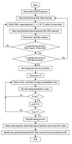
The objective of this work is to design a fractional filter fractional order PID controller for non-integer order plus time delay (NIOPTD) systems using fractional internal model control (IMC) filter structure. The novelty of the work lies in identifying the higher order fractional IMC filter structure using a systematic analytical procedure based on the minimization of integral absolute error (IAE). The resulting controller consists of a fractional filter term and a fractional PID controller. The tuning parameters are identified based on the minimum value IAE for a fixed robustness (Ms). Simulations are carried out for servo and regulatory response and it was found that an enhanced performance is observed with the proposed controller in terms of low IAE and ITAE. Uncertainties in the process parameters are considered to check the robustness and the stability is assessed with robust stability analysis. The results indicate that the closed loop system with the proposed controllers is robustly stable. In addition, fragility analysis has been done for uncertainties in the controller parameters. The major contribution of this work is the analytical design procedure for identification of optimum fractional IMC filter structure with higher order pade’s approximation for timed delay.
internal model control, robustness, fragility, fractional IMC filter structure, uncertainty
The fractional order controllers are gaining wide acceptance in the industrial sector and among the scientific community to control the processes modeled as higher order systems. Higher order models capture the subtleties of the processes and better represent the dynamics of nonlinear processes in a precise manner. It is difficult to control the higher order process models and more challenging if they are associated with time delays. The control performance of such systems degrades if the standard proportional integral derivative (PID) controller is used [1]. This is the concern of many researchers from the last twenty years and this fact resulted in the design and application of fractional order proportional integral derivative (FOPID) controller to improve the closed loop response of time delay systems.
The primary work on fractional order controllers was by Oustaloup in 1991 [2] and subsequently Podlubny [3] proposed an FOPID or PIλDµ controller with the help of fractional calculus. The structure of FOPID controller is such that it becomes a PID controller by setting the fractional powers of integrator and differentiator to unity. This flexibility in the controller structure ensures robust performance of integer order systems and non-integer order systems. Hence, FOPID controller can enhance the closed loop performance of higher order systems. The PIλDµ controller for such systems was developed by approximating higher order systems by lower order time delay systems [4, 5]. Further, the FOPID controller was developed for non-integer order time delay systems as they represent the system dynamics in a better way than integer order systems. Thus, the fractional order PI/PID controller improves the closed loop performance of higher order processes. However, this structure of FOPID controller complicates the tuning with the additional tuning parameters. There are several tuning methods reported in the literature [6] for tuning the FOPID controller and fractional filter PID controller for integer order time delay systems [7-10].
The tuning methods of FOPID controller for fractional order systems gained momentum in the last decade. It has been identified that higher order processes need to be brought to the lower order, preferably of first and second order for frequency domain tuning and time domain tuning of the FOPID controller. Based on this, PIλDµ controller tuning strategies in frequency domain and time domain were proposed for NIOPTD systems [11]. An analytical tuning method of FOPID controller for fractional order systems was proposed after reducing the higher order fractional system by retaining its dynamics [12]. A PIλDµ controller was also designed using soft computing technique for delay free non-integer order systems [13] and by using optimization [14]. The use of IMC [15] method was predominant in the design of FOPID controller for NIOPTD systems [16-18]. The IMC filter used in the IMC method plays a crucial role because the tuning parameters in the IMC based controller are those associated with the IMC filter. The controller in [17] was tuned to meet the specifications such as phase margin, flat phase, gain crossover frequency and infinite gain margin. The controller designed using the method in [18] was tuned based on maximum sensitivity. The aim of the present work is to propose a simple and improved method of designing the FOPID controller using IMC method and fractional IMC filter for NIOPTD systems. The design also includes different approximation for time delay term using Pade’s procedure. The resulting structure of the controller consists of a fractional order PID preceded by fractional filter to provide robust control. The tuning parameters in the controller are associated with fractional filter which are identified through the analytical procedure based on the minimum values of IAE and TV and to meet the maximum sensitivity, Ms specification for fair comparison.
The article is organized as follows: In section 2, the general mathematical representation of fractional order systems is presented along with NIOPTD systems used in this paper. Section 3 presents the IMC based FOPID controller design for NIOPTD systems. The robustness and fragility analysis are briefly described section 4. The simulation results for different NIOPTD processes are presented in section 5 and their closed loop response is compared using various performance indices. Section 6 concludes the paper followed by references.
The dynamics of real time systems are better represented by non-integer order mathematical models using the fractional calculus with the help of fractional integration and differentiation. The fractional order systems are often described by the following fractional order differential equation:
$a_{0} y(t)+\sum_{i=1}^{n} a_{i} D^{a_{i}} y(t)=b_{0} u(t-L)+\sum_{i=1}^{m} b_{i} D^{\beta_{i}} u(t-L)$ (1)
where D is the fractional operator; ai, bi are the real coefficients; αi, βi are the real (R+) orders of fractional derivative; u(t) and y(t) are the real input and output; L is the time delay of the system. The Laplace transform of Eq. (1) produces a fractional order transfer function
$a_{0} Y(s)+\sum_{i=1}^{n} a_{i} S^{\alpha_{i}} Y(s)=b_{0} U(s) e^{-L s}+\sum_{i=1}^{m} b_{i} S^{\beta_{i}} U(s) e^{-L s}$ (2)
where $\mathrm{S}^{\alpha_{\mathrm{i}}} \mathrm{Y}(\mathrm{s})$ and $\mathrm{S}^{\beta_{\mathrm{i}}} \mathrm{U}(\mathrm{s})$ are the Laplace transform of $\mathrm{D}^{\alpha_{\mathrm{i}}} \mathrm{y}(\mathrm{t}) \cdot$ and $\cdot \mathrm{D}^{\beta_{\mathrm{i}} \mathrm{u}(\mathrm{t})}$ respectively. Then, the transfer function of non-integer order system is
$\mathrm{G}(\mathrm{s})=\frac{\mathrm{Y}(\mathrm{s})}{\mathrm{U}(\mathrm{s})}=\frac{\mathrm{b}_{0}+\sum_{\mathrm{i}=1}^{\mathrm{m}} \mathrm{b}_{\mathrm{i}} \mathrm{S}^{\beta_{\mathrm{i}}}}{\mathrm{a}_{0}+\sum_{\mathrm{i}=1}^{\mathrm{n}} \mathrm{a}_{\mathrm{i}} \mathrm{S}^{\alpha_{\mathrm{i}}}} \mathrm{e}^{-\mathrm{L} \mathrm{s}}$ (3)
The fractional operators $\mathrm{S}^{\alpha_{\mathrm{i}}}$ and $\mathrm{S}^{\beta_{\mathrm{i}}}$ are difficult to program for simulations and for practical implementation in the hardware. Though, there are several means of practical implementation of fractional operators the most widely used one is the approximation of the fractional operator by integer order transfer function. The popular approximation used for fractional operator was by Oustaloup recursive filter [2] which is based on the recursive distribution of poles and zeros over a frequency range [ωl, ωh]. This filter is given by
$\mathrm{S}^{\mathrm{v}}=\mathrm{K} \prod_{\mathrm{k}=-\mathrm{N}}^{\mathrm{N}} \frac{\mathrm{s}+\omega_{\mathrm{k}}^{\prime}}{\mathrm{s}+\omega_{\mathrm{k}}}$ (4)
where N is the number of poles and zeros. Selection of N is crucial for the approximation; smaller values of N results in ripples in the gain and phase behavior, but they are minimized for higher values of N causing an increase in the computational load. The poles, zeros and gain are evaluated using the following Equations:
$\omega_{\mathrm{k}}^{\prime}=\omega_{1}\left(\frac{\omega_{\mathrm{h}}}{\omega_{1}}\right)^{\left(\mathrm{k}+\mathrm{N}+\frac{1-v}{2}\right) /(2 \mathrm{N}+1)}$ (5a)
$\omega_{\mathrm{k}}=\omega_{1}\left(\frac{\omega_{\mathrm{h}}}{\omega_{1}}\right)^{\left(\mathrm{k}+\mathrm{N}+\frac{1+v}{2}\right) /(2 \mathrm{N}+1)}$ (5b)
$\mathrm{K}=\omega_{\mathrm{h}}^{\mathrm{v}}$ (5c)
The non-integer order process models used for the design of FOPID controller are:
(1) One non-integer order plus time delay (NIOPTD-I) system
$\mathrm{G}_{\mathrm{m}}(\mathrm{s})=\frac{\mathrm{K}}{\mathrm{Ts}^{\alpha}+1} \mathrm{e}^{-\mathrm{L} \mathrm{s}}$ (6)
where K-system gain; L-time delay; T-time constant and α-fractional order.
Two cases of NIOPTD-I process [18] are possible based on the value of α: case I (0<α<1); case II (1≤α<2).
(2) Two non-integer order plus time delay (NIOPTD-II) system
$\mathrm{G}_{\mathrm{m}}(\mathrm{s})=\frac{\mathrm{K}}{\mathrm{s}^{\alpha}+2 \zeta \omega_{\mathrm{n}} \mathrm{s}^{\beta_{+}} \omega_{\mathrm{n}}^{2}} \mathrm{e}^{-\mathrm{L} \mathrm{s}}$ (7)
where α and β are the flexible system orders. This flexibility allows the accurate modeling of the processes with minimum modeling error compared to first order and second order time delay (FOPTD and SOPTD) models. The two cases of NIOPTD-II process based on the value of α and β are: case I (1<α<2, α>β) and case II (2≤α<3, α>β).
3.1 Internal model control
The block diagram of IMC control structure and its equivalent feedback control structure is shown in Figure 1.
Figure 1. Block diagram (a) IMC scheme (b) feedback loop
The IMC controller design procedure is summarized as follows:
Step 1: Divide the process model into noninvertible and invertible parts
$\mathrm{G} _ {\mathrm{m}} (\mathrm{s}) = \mathrm {G} _ {\mathrm {m}} ^ {+} (\mathrm{s}) \ mathrm{G} _ {\mathrm{m}} ^ {-} (\mathrm{s})$ (8)
where $\mathrm{G}_{\mathrm{m}}^{+}(\mathrm{s})$ consists of all time delays and right-half plane zeros. $\mathrm{G}_{\mathrm{m}}^{-}(\mathrm{s})$ is invertible and contains minimum phase elements.
Step 2: Obtain the IMC controller by adding a low-pass filter whose structure must be selected such that IMC controller is proper.
$\mathrm {C} _ {\mathrm{IMC}} (\mathrm{s}) = \left[\mathrm{G} _ {\mathrm{m}} ^ {-} (\mathrm{s}) \right] ^ {-1} \mathrm{f} (\mathrm{s})$ (9)
where f(s) is the IMC filter
Step 3: The feedback controller C(s) is
$\mathrm {C} ( \mathrm{s}) = \frac {\mathrm {C} _ { \mathrm {IMC}} ( \mathrm{s}) } { 1-\mathrm {C} _ { \mathrm{IMC} } ( \mathrm {s}) \ mathrm {G} (\mathrm{s}) } $ (10)
3.2 Proposed design
The proposed fractional filter fractional order PID controller structure is
$ \mathrm {C} ( \mathrm {s}) = ( \text { fractional filter term }) \mathrm {K} _ {\mathrm{p}} \left [1+ \frac{1} { \mathrm{T} _ { \mathrm{i}} \mathrm{s} ^ {2}}+ \mathrm {T} _ {\mathrm {d}} \mathrm {s} ^ { \mu}\right]$ (11)
The fractional IMC filter structures used in the present design are:
$\mathrm {f} (\mathrm{s}) = \frac {1} {\left(\gamma \mathrm{s} ^ {\mathrm{p}+1} \right) ^ {\mathrm{n}}} ; \mathrm{n} = 1,2,3$ (12)
$\mathrm {f} ( \mathrm{s}) = \frac {\eta \mathrm{s}+1} { \left( \gamma \ mathrm {s} ^ {\mathrm {p}}+ 1 \right ) ^ { \mathrm {n}+1}} ; \mathrm {n}=1,2$ (13)
$\mathrm{f} ( \mathrm{s})= \frac{ (\eta \mathrm {s}+1) ^ {2}} {\left(\gamma \mathrm{s} ^ {\mathrm {p} }+ 1\right) ^ {\mathrm {n} +2}} ; \mathrm {n} =1,2$ (14)
γ is the filter time constant, p is the fractional order and η is the additional degree of freedom.
The fractional IMC filter controller according to Eq. (9) for the NIOPTD-I system defined in Eq. (6) and by using fractional IMC filter structure defined in Eq. (12) is
$\mathrm {C} _ {\mathrm{IMC}} (\mathrm{s}) = \left(\frac {\mathrm {Ts} ^ {\alpha _ {+}} +1} {\mathrm {K}} \right) \frac {1} {\left(\gamma \mathrm {s} ^ {\mathrm {p} } +1 \right)^{\mathrm {n} }}$ (15)
The feedback controller using fractional IMC filter is
$C(s)= \frac {T s ^ {\alpha} +1} {K\left [\left(\gamma s^ {p} + 1\right) ^ {n} -e ^ {-L s} \right]} $ (16)
Now, by using Pade's procedure for $e^{-L s}$ (Table 1), the general expression for C(s) is
$\mathrm {C} (\mathrm {s}) = (\text { fractional filter term } ) \left ( \frac{ \mathrm {T} } { \mathrm {K} } \right) \left (1+ \frac {1} { \mathrm {Ts} ^ {a}} \right)$ (17)
It can be observed from Eq. (17) that the controller is composed of fractional PI term in series with fractional filter term. Similarly, the controller is derived for other fractional IMC filter structures (Eq. (13) & Eq. (14)) by following the above design procedure (steps). The resulting controller takes the form given in Eq. (17). All the controllers derived using different fractional IMC filter structures differ only in the fractional filter term.
The feedback controller for NIOPTD-II process can be obtained by applying the same procedure used for NIOPTD-I process. The generalized controller equation for all fractional IMC filter structures is
$\mathrm {C} (\mathrm {s})=(\text { fractional filter term }) \left ( \frac {2 \zeta \omega_ {n}} {\mathrm {K}} \right) \left (1+ \frac {\omega _ {\mathrm {n}}} {2 \zeta \mathrm {s} ^ {\beta}}+ \frac {1} {2 \zeta \omega_{\mathrm {n}}} \mathrm {s} ^ {\alpha- \beta} \right)$ (18)
Table 1. Equivalent term of $e^{-L s}$ using Pade’s procedure
|
1st Pade |
1/2 Pade |
2nd Pade |
2/3 Pade |
|
$\frac{1-0.5 \mathrm{Ls}}{1+0.5 \mathrm{Ls}}$ |
$\frac{6-2 \mathrm{Ls}}{6+4 \mathrm{Ls}+\mathrm{L}^{2} \mathrm{s}^{2}}$ |
$\frac{1-(\mathrm{L} / 2) \mathrm{s}+\left(\mathrm{L}^{2} / 12\right) \mathrm{s}}{1+(\mathrm{L} / 2) \mathrm{s}+\left(\mathrm{L}^{2} / 12\right)}$ |
$\frac{60-24 \mathrm{Ls}+3 \mathrm{L}^{2} \mathrm{s}^{2}}{60+36 \mathrm{Ls}+9 \mathrm{L}^{2} \mathrm{s}^{2}+\mathrm{L}^{3} \mathrm{s}}$ |
4.1 Robustness analysis
The closed loop stability must be assessed for the nominal process conditions and with uncertainties in the processes. This is verified with a robust stability condition [19].
$\left\|_{\mathrm{m}}(\mathrm{j} \omega) \mathrm{T}(\mathrm{j} \omega)\right\|<1 \forall \omega \in(-\infty, \infty)$ (19)
where $\mathrm{T}(\mathrm{s})_{\mathrm{s}=\mathrm{j} \omega}=\frac{\mathrm{C}(\mathrm{s}) \mathrm{G}(\mathrm{s})}{1+\mathrm{C}(\mathrm{s}) \mathrm{G}(\mathrm{s})}$ - the complementary sensitivity function; $l_{\mathrm{m}}(\mathrm{j} \omega)=\left|\frac{\mathrm{G}(\mathrm{j} \omega)-\mathrm{G}_{\mathrm{m}}(\mathrm{j} \omega)}{\mathrm{G}_{\mathrm{m}}(j \omega)}\right|$ - Process multiplicative uncertainty bound.
Using robust stability analysis, one can know the amount of uncertainty that can be introduced into the process parameters for the robust performance once the controller is designed. The controller must be tuned according to Eq. (20) for uncertainty in L
$\|\mathrm{T}(\mathrm{j} \omega)\|_{\infty}<\frac{1}{\left|\mathrm{e}^{-\Delta \mathrm{L}}-1\right|}$ (20)
4.2 Fragility analysis
The robust performance of the closed loop system should also be observed for changes in controller parameters. This is found through loss of robustness (Ms) of the system using fragility analysis [20]. The degree of controller fragility is decided based on robustness delta 20 fragility index (RFIΔ20) which is defined in Eq. (21)
$\mathrm{RFI}_{\Delta 20}=\frac{\mathrm{M}_{\mathrm{s} \Delta 20}}{\mathrm{M}_{\mathrm{s}}}-1$ (21)
MsΔ20 is the Ms for 20 % variation in all parameters of the controller and Ms in the nominal maximum sensitivity. Any controller is said to be resilient if $\mathrm{RFI}_{\Delta 20} \leq 0.1$ nonfragile if $0.1<\mathrm{RFI}_{\Delta 20} \leq 0.5$ and fragile if $\mathrm{RFI}_{\Delta 20}>0.5$.
The effectiveness of the proposed fractional filter FOPID controller is explained with four examples representing all cases of NIOPTD system. The control scheme used is the feedback loop shown in Figure 1. The simulations have been performed for a step change in set point and disturbance. The system's performance is also observed for perturbations (-20 % in K and +10 % in L) in the process parameters and for Gaussian noise in the output. The closed loop performance of the NIOPTD system is assessed by using the performance measures given in Table 2.
Table 2. Performance measures
|
IAE |
ITAE |
TV |
Ms |
|
$\int_{0}^{\infty}|e(t)| d t$ |
$\int_{0}^{\infty} t|e(t)| d t$ |
$\sum_{i=0}^{\infty}\left|u_{i+1}-u_{i}\right|$ |
$\max _{0<\omega<\infty}\left|\frac{1}{1+C(j \omega) G(j \omega)}\right|$ |
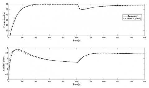
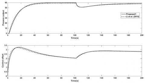
The frequency used for Oustaloup filter approximation of fractional operator is 0.001-1000rad/s. The Proposed1 controller settings are listed in Table 4. The closed loop step response with a disturbance of magnitude -1 applied at t=100s is shown in Figure 3. The corresponding performance measures are given in Table 5. It is evident that the Proposed1 method gives improved performance with low IAE, ITAE and TV compared to Li et al. method [18]. The perturbed response and the associated performance measures are presented in Figure 4 and Table 6. The Proposed1 method clearly gives better result than the method used for comparison. The IAE and ITAE values for the response in presence of output noise of variance 10 given in Table 7 are close to each other for both the methods but the TV value is low with the Proposed1 method.
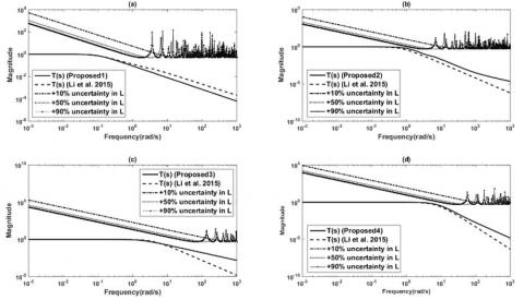
The robust stability of the closed loop system is assessed with magnitude plot for T(s). The magnitude plot for the current example is shown in Figure 5. It is observed that both the methods are robustly stable up to +90 % uncertainty in L obeying the robust stability condition (Eq. 20).
Figure 3. Nominal response of Example 1
Table 3. Fractional filter terms of the optimum controller
|
Process |
Fractional filter term |
|
NIOPTD-I (case I) |
$\frac{\mathrm{L}^{3} \mathrm{s}^{3}+9 \mathrm{L}^{2} \mathrm{s}^{2}+36 \mathrm{Ls}+60}{\left(\gamma \mathrm{L}^{3} \mathrm{s}^{\mathrm{p}+2}+9 \gamma \mathrm{L}^{2} \mathrm{s}^{\mathrm{p}+1}+\mathrm{L}^{3} \mathrm{s}^{2}+36 \gamma \mathrm{L} \mathrm{s}^{\mathrm{p}}+6 \mathrm{L}^{2} \mathrm{s}+60 \gamma \mathrm{s}^{\mathrm{p}-1}+60 \mathrm{L}\right) \mathrm{s}^{1-\alpha}}$ |
|
NIOPTD-I (case II) |
$\frac{\eta^{3} L^{3} s^{5}+\left(9 \eta^{2} L^{2}+2 \eta L^{3}\right) s^{4}+\left(36 \eta^{2} L+18 \eta L^{2}+L^{3}\right) s^{3}+\left(60 \eta^{2}+72 \eta L+9 L^{2}\right) s^{2}+(36 L+120 \eta) s+60}{(\gamma^{3} L^{3} s^{3 p+2}+9 \gamma^{3} L^{2} s^{3 p+1}+3 \gamma^{2} L^{3} s^{2 p+2}+36 \gamma^{3} L s^{3 p+2} 7 \gamma^{2} L^{2} s^{2 p+1}+3 \gamma L^{3} s^{p+2}-3 \eta^{2} L^{2} s^{3}+60 \gamma^{3} s^{3 p-1}+108 \gamma^{2} L s^{2 p}+27 \gamma \mathrm{L}^{2} \mathrm{s}^{\mathrm{p}+1}+\left(\mathrm{L}^{3}+24 \eta^{2} \mathrm{L}-6 \eta \mathrm{L}^{2}\right) \mathrm{s}^{2}+180 \gamma^{2} \mathrm{s}^{2 \mathrm{p}-1}+108 \gamma \mathrm{L} \mathrm{s}^{\mathrm{p}}+\left(48 \eta L+6 L^{2}-60 \eta^{2}\right) s+180 \gamma s^{p-1}+(60 L-120 \eta))s^{1-a}}$ |
|
NIOPTD-II (case I) |
$\frac{L^{3} s^{3}+9 L^{2} s^{2}+36 L s+60}{\left(\gamma L^{3} s^{p+2}+9 \gamma L^{2} s^{p+1}+L^{3} s^{2}+36 \gamma L s^{p}+6 L^{2} s+60 \gamma s^{p-1}+60 L\right) s^{1-\beta}}$ |
|
NIOPTD-II (case II) |
$\frac{$\eta L^{3} s^{4}+\left(9 \eta L^{2}+L^{3}\right) s^{3}+\left(36 \eta L+9 L^{2}\right) s^{2}+(36 L+60 \eta) s+60$}{(\gamma^{3} \mathrm{L}^{3} \mathrm{s}^{3} \mathrm{p}+2+9 \gamma^{3} \mathrm{L}^{2} \mathrm{s}^{3 \mathrm{p}+1}+3 \gamma^{2} \mathrm{L}^{3} \mathrm{s}^{2 \mathrm{p}+2}+36 \gamma^{3} \mathrm{L} \mathrm{s}^{3 \mathrm{p}+27 \gamma^{2} \mathrm{L}^{2} \mathrm{s}^{2 \mathrm{p}+1}}+3 \gamma L^{3} s^{p+2}+60 \gamma^{3} s^{3 p-1}+108 \gamma^{2} L s^{2 p}+27 \gamma \mathrm{L}^{2} \mathrm{s}^{\mathrm{p}+1}+\left(\mathrm{L}^{3}-3 \eta \mathrm{L}^{2}\right) \mathrm{s}^{2}+180 \gamma^{2} \mathrm{s}^{2 \mathrm{p}-1}+108 \gamma \mathrm{Ls}^{\mathrm{p}}+\left(24 \eta \mathrm{L}+6 \mathrm{L}^{2}\right) \mathrm{s}+180 \gamma \mathrm{s}^{\mathrm{p}-1}+(60 \mathrm{L}-60 \eta))s^{1-β}}$ |
|
Example |
Kp |
Ti |
λ |
Td |
µ |
η |
γ |
p |
Ms |
|
Example 1 |
0.19 |
12.72 |
0.5 |
- |
- |
- |
11.1 |
1.05 |
1.15 |
|
Example 2 |
0.3 |
1.5 |
1.5 |
- |
- |
0.2 |
0.66 |
1.01 |
1.51 |
|
Example 3 |
1.1963 |
1.1964 |
0.9997 |
0.1648 |
0.9947 |
- |
0.53 |
1.03 |
1.04 |
|
Example 4 |
1.17 |
1.17 |
1.02 |
0.1912 |
1.45 |
0.03 |
0.1085 |
1.02 |
1.49 |
|
Examples |
Method |
Servo response |
Regulatory response |
Ms |
||||
|
|
|
IAE |
ITAE |
TV |
IAE |
ITAE |
TV |
|
|
Example 1 |
Proposed1 |
694.1 |
6650 |
4.128 |
365.2 |
11780 |
1.0046 |
1.15 |
|
Li et al. [18] |
716 |
9410 |
4.334 |
370 |
12680 |
1.323 |
1.15 |
|
|
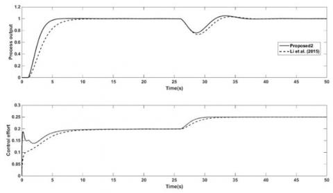
Example 2 |
Proposed2 |
2.576 |
3.28 |
0.355 |
0.9444 |
1.667 |
0.1093 |
1.51 |
|
Li et al. [18] |
3.502 |
7.663 |
0.2008 |
1.095 |
3.057 |
0.0644 |
1.51 |
|
|
Example 3 |
Proposed3 |
0.5756 |
0.2764 |
19.794 |
0.2791 |
0.4618 |
0.5014 |
1.04 |
|
Li et al. [18] |
0.581 |
0.2771 |
4.987 |
0.2801 |
0.4531 |
0.4979 |
1.04 |
|
|
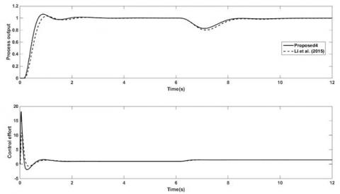
Example 4 |
Proposed4 |
0.4761 |
0.0483 |
42.56 |
0.2009 |
0.2773 |
0.6106 |
1.49 |
|
Li et al. [18] |
0.5383 |
0.1384 |
25.037 |
0.2506 |
0.3776 |
0.5779 |
1.49 |
|
|
Examples |
Method |
Servo response |
|
Regulatory response |
||||
|
|
|
IAE |
ITAE |
TV |
|
IAE |
ITAE |
TV |
|
Example 1 |
Proposed1 |
866.1 |
10480 |
4.524 |
|
361.2 |
12380 |
1.0002 |
|
Li et al. [18] |
890.5 |
13740 |
4.7928 |
|
364.7 |
13170 |
1.4437 |
|
|
Example 2 |
Proposed2 |
3.184 |
5.784 |
0.3817 |
|
0.82 |
2.069 |
0.1115 |
|
Li et al. [18] |
4.378 |
12.97 |
0.2535 |
|
0.9372 |
3.815 |
0.0596 |
|
|
Example 3 |
Proposed3 |
0.718 |
0.4431 |
19.5423 |
|
0.2776 |
0.4935 |
0.4999 |
|
Li et al. [18] |
0.7244 |
0.4378 |
4.7374 |
|
0.2784 |
0.4838 |
0.4968 |
|
|
Example 4 |
Proposed4 |
0.5371 |
0.1067 |
41.5226 |
|
0.201 |
0.2978 |
0.5294 |
|
Li et al. [18] |
0.6404 |
0.2446 |
24.4893 |
|
0.2504 |
0.4076 |
0.5098 |
|
|
Examples |
Method |
Servo response |
|
Regulatory response |
||||
|
|
|
IAE |
ITAE |
TV |
|
IAE |
ITAE |
TV |
|
Example 1 |
Proposed1 |
244 |
398.3 |
5.4628 |
|
436.5 |
12070 |
5.803 |
|
Li et al. [18] |
245.3 |
463.3 |
8.7353 |
|
435.6 |
12990 |
9.1528 |
|
|
Example 2 |
Proposed2 |
3.184 |
3.091 |
0.5316 |
|
1.436 |
1.417 |
0.2929 |
|
Li et al. [18] |
4.019 |
7.183 |
0.2699 |
|
1.532 |
2.566 |
0.1306 |
|
|
Example 3 |
Proposed3 |
0.6153 |
0.615 |
22.644 |
|
0.2767 |
0.411 |
3.3611 |
|
Li et al. [18] |
0.615 |
0.228 |
5.6143 |
|
0.287 |
0.4039 |
1.1652 |
|
|
Example 4 |
Proposed4 |
0.5332 |
0.1088 |
50.158 |
|
0.245 |
0.3379 |
8.5352 |
|
Li et al. [18] |
0.6164 |
0.2108 |
29.530 |
|
0.2951 |
0.4501 |
5.1956 |
|
Table 8. Robustness delta 20 (RFIΔ20) fragility index for all the examples
|
Example 1 |
Example 2 |
||
|
Proposed1 |
0.1513 |
Proposed2 |
3.5165 |
|
Li et al. [18] |
0.0035 |
Li et al. [18] |
0.6874 |
|
Example 3 |
Example 4 |
||
|
Proposed3 |
0.0027 |
Proposed4 |
3.604 |
|
Li et al. [18] |
0.1 |
Li et al. [18] |
0.4697 |
In this paper, an improved analytical design of the FOPID controller is proposed for non-integer order plus time delay systems after identifying the optimum fractional IMC filter based on minimum IAE for a fixed Ms. The proposed method enhances the closed loop performance with additional tuning parameters in the controller design. Improved step response is observed for different input changes on the closed loop system. Improvement is observed with the controller designed using 2/3 order Pade’s approximation for time delay. The error values are decreasing with the proposed controller for all the NIOPTD processes but the control effort is increasing with increase in the order of approximation. All the proposed methods give robust and stable performance for parametric uncertainty. The fractional controllers have become fragile for uncertainties in the controller parameters when higher order fractional IMC filter is used during their design. Hence, attention should be needed while changing the fractional orders of the controller and filter. Fragility analysis in presence of process parametric uncertainties can be taken up as a future work. The proposed method can be extended to design fractional controller for unstable non integer order systems.
|
G |
process model |
|
C |
controller |
|
f T |
IMC filter complementary sensitivity function |
|
L RFI M D S Y U K L T |
process multiplicative uncertainty bound robustness fragility index maximum sensitivity fractional operator Laplace transform of D process output process input system gain time delay time constant |
|
Greek symbols |
|
|
a |
fractional order |
|
b ω |
fractional order frequency |
|
ζ λ μ |
damping coefficient fractional order of integrator fractional order of differentiator |
|
γ |
IMC filter time constant |
|
η |
additional degree of freedom |
|
Subscripts |
|
|
p |
proportional |
|
i |
integral |
|
d m n l h |
derivative model natural low high |
[1] Vilanova, R., Visioli, A. (2012). PID control in the third millennium. London: Springer. https://doi.org/10.1007/978-1-4471-2425-2
[2] Oustaloup, A. (1991). La commande CRONE: commande robusted'ordre non entier. Hermes.
[3] Podlubny, I. (1999). Fractional-order systems and PIλDµ controllers. IEEE Transactions on Automatic control, 44(1): 208-214. https://doi.org/10.1016/j.camwa.2013.02.015
[4] Monje, C.A., Vinagre, B.M., Feliu, V., Chen, Y. (2008). Tuning and auto-tuning of fractional order controllers for industry applications. Control Engineering Practice, 16(7): 798-812. https://doi.org/10.1016/j.conengprac.2007.08.006
[5] Padula, F., Visioli, A. (2011). Tuning rules for optimal PID and fractional-order PID controllers. Journal of Process Control, 21(1): 69-81. https://doi.org/10.1016/j.jprocont.2010.10.006
[6] Shah, P., Agashe, S. (2016). Review of fractional PID controller. Mechatronics, 38: 29-41. https://doi.org/10.1016/j.jprocont.2010.10.006
[7] Ranganayakulu, R., Babu, G.U., Rao, A.S., Patle, D.S. (2016). A comparative study of fractional order PIλ/PIλDµ tuning rules for stable first order plus time delay processes. Resource Efficient Technologies, 2: S136-52. https://doi.org/10.1016/j.reffit.2016.11.009
[8] Sánchez, H.S., Padula, F., Visioli, A., Vilanova, R. (2017). Tuning rules for robust FOPID controllers based on multi-objective optimization with FOPDT models. ISA Transactions, 66: 344-361. https://doi.org/10.1016/j.isatra.2016.09.021
[9] Ranganayakulu, R., Babu, G.U.B., Rao, A.S. (2018). Analytical design of Enhanced Fractional filter PID controller for improved disturbance rejection of second order plus time delay processes. Chemical Product and Process Modeling, 14(1). https://doi.org/10.1515/cppm-2018-0012
[10] Padula, F., Visioli, A. (2013). Set-point weight tuning rules for fractional-order PID controllers. Asian Journal of Control, 4: 1-13. https://doi.org/10.1002/asjc.634
[11] Das, S., Saha, S., Das, S., Gupta, A. (2011). On the selection of tuning methodology of FOPID controllers for the control of higher order processes. ISA Transactions, 50(3): 376-388. https://doi.org/10.1016/j.isatra.2011.02.003
[12] Tavakoli-Kakhki, M., Haeri, M. (2011). Fractional order model reduction approach based on retention of the dominant dynamics: Application in IMC based tuning of FOPI and FOPID controllers. ISA Transactions, 50(3): 432-442. https://doi.org/10.1016/j.isatra.2011.02.002
[13] Liu, L., Pan, F., Xue, D. (2015). Variable-order fuzzy fractional PID controller. ISA Transactions, 55: 227-233. https://doi.org/10.1016/j.isatra.2014.09.012
[14] Zeng, G.Q., Chen, J., Dai, Y.X., Li, L.M., Zheng, C.W., Chen, M.R. (2015). Design of fractional order PID controller for automatic regulator voltage system based on multi-objective extremal optimization. Neurocomputing, 160: 173-184. https://doi.org/10.1016/j.neucom.2015.02.051
[15] Shamsuzzoha, M., Skliar, M., Lee, M. (2012). Design of IMC filter for PID control strategy of open-loop unstable processes with time delay. Asia-Pacific Journal of Chemical Engineering, 7: 93-110. https://doi.org/10.1002/apj.497
[16] Vinopraba, T., Sivakumaran, N., Narayanan, S., Radhakrishnan, T.K. (2012). Design of internal model control based fractional order PID controller. Journal of Control Theory and Applications, 10(3): 297-302. https://doi.org/10.1007/s11768-012-1044-4
[17] Bettayeb, M., Mansouri, R. (2014). Fractional IMC-PID-filter controllers design for non integer order systems. Journal of Process Control, 24(4): 261-271. https://doi.org/10.1016/j.jprocont.2014.01.014
[18] Li, D., Liu, L., Jin, Q., Hirasawa, K. (2015). Maximum sensitivity based fractional IMC–PID controller design for non-integer order system with time delay. Journal of Process Control, 31: 17-29. https://doi.org/10.1016/j.jprocont.2015.04.001
[19] Morari, M., Zafiriou, E. (1989). Robust Process Control. Prentice hall: Englewood Cliffs, NJ.
[20] Alfaro, V.M., Vilanova, R. (2012). Fragility evaluation of PI and PID controllers tuning rules. In PID control in the third millennium. Springer: London, 349-380. https://doi.org/10.1007/978-1-4471-2425-2_12
[21] Malek, H., Luo, Y., Chen, Y. (2013). Identification and tuning fractional order proportional integral controllers for time delayed systems with a fractional pole. Mechatronics, 23(7): 746-754. https://doi.org/10.1016/j.mechatronics.2013.02.005
[22] Das, S., Pan, I., Das, S. (2013). Performance comparison of optimal fractional order hybrid fuzzy PID controllers for handling oscillatory fractional order processes with dead time. ISA Transactions, 52(4): 550-566. https://doi.org/10.1016/j.isatra.2013.03.004
[23] Pan, I., Das, S. (2013). Model reduction of higher order systems in fractional order template. In Intelligent Fractional Order Systems and Control, Springer: Berlin Heidelberg, pp. 241-256. https://doi.org/10.1007/978-3-642-31549-7_9