Bnan Al-Qallab* | Hamzeh Duwairi
OPEN ACCESS
The objective of this work is to model the fluctuating air stream potential of producing wind energy and study different operating parameters of wind turbines, by using conservation principles continuity and momentum, with wind turbine equations. A combination of two numerical methods which include Runge-Kuttha technique with shooting technique were utilized using MATLAB to obtain numerical solutions. It is found that the increasing of corrugated surface amplitudes decreases velocities inside boundary layers and reduce power output compared to those obtained by Blasius or traditional Pet theory.
boundary layer, electricity production, surface topography, velocity fluctuations, wind energy
Considering steady state wind loads for short periods can incorporate steady state wind model. In addition, the involving of incompressible wind model is usual; this is due to small forces of wind compared to a ramjet or turbojet.
2.1 Governing equations
The corrugated surface can be described by the following equation:
$y=σ(x)=asin(\frac{2πx}{λ})$ (1)
where a*is the amplitude of the wavy surface. It may take values from zero to one and even greater than 1 because it reflects -in physics- the height of hills or buildings relative to distance between them. If a is greater than one; forests of trees near each other are considered, if it is smaller than one; distributed or extended hills are considered, λ is the characteristic length associated with the wave and is the surface profile of the tidal waves.
The laminar boundary-layer governing equations are:
The continuity equation:
$\frac{∂u}{∂x}+\frac{∂v}{∂y}=0$ (2)
The x-momentum equation:
$u\frac{∂u}{∂x}+v\frac{∂u}{∂y}=-\frac{1}{ρ}\frac{∂p}{∂x}+v(\frac{∂^2u}{∂x^2}+\frac{∂^2u}{∂y^2})$ (3)
The y-momentum equation:
$u\frac{∂v}{∂x}+v\frac{∂v}{∂y}=-\frac{1}{ρ}\frac{∂p}{∂y}+v(\frac{∂^2v}{∂x^2}+\frac{∂^2v}{∂y^2})$ (4)
This is a system of elliptic, nonlinear partial differential equations of the second order. They are accompanied by initial and boundary conditions. Here u, v are the axial and normal velocity components in the x and y directions respectively, p is the fluid pressure and v is the Kinematic viscosity which equals ($v=\frac{u}{ρ}$).
The corresponding boundary conditions for the present problem are:
$u=0$, $v=0$ at $y=0$
$u=u∞$ at $y→∞$ (5)
Here, the following non-dimensional variables are:
$y*=y-σ(x)$ $x*=\frac{x}{λ}$
$a*=\frac{a}{λ}$ $v*=v-λxu$ $u*=u$ (6)
The flow is governed by the following dimensionless form of the governing equations after using the proper non-dimensional transformation variables (6) which can be written as:
The x-momentum equation:
$u*\frac{∂u*}{∂x*}+v*\frac{∂u*}{∂y*}=\frac{1}{ρ}\frac{∂p}{∂y*}σx+(1+σx^2)\frac{∂^2u*}{∂y*^2}$ (7)
The y-momentum equation:
$σx(u*\frac{∂u*}{∂x*}+v*\frac{∂u*}{∂y*})=-\frac{1}{ρ}\frac{∂p}{∂y*}+vσx(1+σx^2)\frac{∂^2u*}{∂y*^2}-σxxu*^2$ (8)
By Combining equations (7) and (8) and eliminating $\frac{∂p}{∂y}$ from them, the resultant equation is expressed as follows:
$u*\frac{∂u*}{∂x*}+v*\frac{∂u*}{∂y*}=v(1+σx^2)\frac{∂^2u*}{∂y*^2}-\frac{σxσxxu*^2}{1+σx^2}$ (9)
where, $σx=\frac{dσ(x)}{dx}$, $σxx=\frac{d^2σ(x)}{dx^2}$
Then, the following transformations are introduced and the use of well-known relations between velocity components u, v and stream function ψ is integrated, in order to reduce the boundary layer equation to an equation with a single dependent variable by changing the partial differential equation (PDE) to ordinary differential equation (ODE), let:
$η=\sqrt{\frac{u∞}{vx}}y$, $ψ(x,y)=\sqrt{u∞vx}f(η)$ (10)
where, η is a similarity variable and ψ is the stream function.[17] The transformations given in Equation (10) are introduced into Equation (9), the momentum equation is transformed to the following form:
$(1+σx^2)f'''+\frac{1}{2}ff''-\frac{σxσxx}{1+σx^2}xf'^2=0$ (11)
The corrugated surface function transformation to non-dimensional derivatives is represented as follows:
$y=σ(x)=asin\frac{2πx}{λ}$
$σ*(x)=σ(x)$ (12)
$σx*=σx$ (13)
$\frac{σxx*}{λ}=σxx$ (14)
That results in the following resultant equation:
$f'''-\frac{σx*σxx*}{(1+σx*2)^2}x*f'^2+\frac{1}{2(1+σx*^2)}ff''=0$ (15)
The boundary conditions associated by equation (2.15) take the following form:
$f(η)=0$, $f'(η)=0$ at $η=0$
$f'(η)=1$ at $η=∞$ (16)
The following equations are used to calculate $η_1$, $η_2$ at specific Rex, y and x.
$η_1=\frac{y_1}{x}\sqrt{Rex}$ (17)
$η_2=\frac{y_2}{x}\sqrt{Rex}$ (18)
where, x* is the distance along corrugated surface as dimensionless distance, it describes the shape of corrugated surface as it ends on x*, it also ranges from (0-1), x is the dimensional distance on earth, $y_1$ equals the hub height minus the turbine radius, and $y_2$ is the hub height plus the radius.
2.2 Power calculations
The actual wind power extracted by the rotor blades can be calculated under the effect of a corrugated surface using the following resultant formula.
The general power equation is represented below [18].
$P(u(0,R))=\frac{1}{2}ρAu^3(0,R)Cp$
$P=\int_A\frac{1}{2}ρu^3CpdA=\int^{y_2}_{y_1}\frac{1}{2}ρu^3CPdy$ (19)
The potential power is calculated by considering the integration on turbine blades center to outside radius where area is (2πrdr) and the radius changes from 0 to R Which can be expressed as the area enclosed by $f'$(η) curve and limited by the turbine swept area.
$u=u∞f'(η)η=\frac{y}{x}\sqrt{Rex}\to dη=\frac{dy}{x}\sqrt{Rex}$
$P=\int^{η_2}_{η_1}\frac{1}{2}ρu∞^3\frac{x}{\sqrt{Rex}}f'^3(η)dη$ (20)
$P\frac{\sqrt{Rex}}{\frac{ρu∞^3x}{2}}=\int^{η_2}_{η_1}f'^3(η)dη$
The non-dimensional wind power is expressed as follows:
$P*=\int^{η_2}_{η_1}f'^3(η)dη$ (21)
Another power terms must be introduced here ̏ pet power ̋ as the power calculated by substituting freestream velocity outside BL, it is the power of the freestream without involving BL and the associated friction effects.
$Ppet=0.5*ρ*U∞^3*Cp$ (22)
That results in the upcoming non-dimensional term of power: $P*=\frac{P}{Ppet}$
And ̏ Blasius power ̋ when talking about two-dimensional steady flow of an incompressible constant property fluid over a semi-infinite flat plate. So calculating power ratio according to Blasius will have the following formula:
$P*=\frac{P}{PBlasius}=\frac{\int^{η_2}_{η_1}f'^3(η)dη}{\int^{η_2}_{η_1}f'^3(η)dη}$ (23)
Tip-Speed-Ratio (TSR) can be calculated based on radius (R), rotational speed or rotor tip speed (ω) of an elected wind turbine and wind velocity. The following formulas will simplify the equations for calculating TSR.
Wind velocity $U=\int^{η_2}_{η_1}f'(η)dη$
$TSR=\frac{w*R}{U}$ (24)
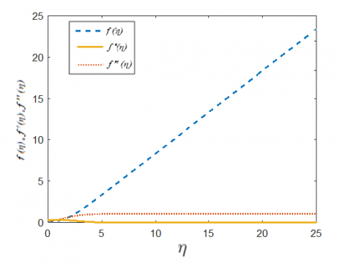
Figure 1. The dimensionless velocity f ʹ(η), sheer stress f ʹʹ (η) and stream function f(η) profiles when x*=0.5 and a*=0
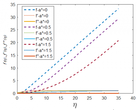
Figure 2. The dimensionless velocity f ʹ(η), sheer stress f ʹʹ (η) and stream function f(η) profiles for different values of a*=(0,0.5,1.5) and x*=0.5
Figure 3. The dimensionless velocity f ʹ(η), sheer stress f ʹʹ (η) and stream function f(η) profiles for different values of a*= (0.2, 0.75) and x*=0.5
Figure 4. The dimensionless velocity f ʹ(η), sheer stress f ʹʹ (η) and stream function f(η) profiles with respect to (η) when x*= (0.25, 0.75) and a*=0.1
Figure 5. The dimensionless velocity f ʹ(η), sheer stress f ʹʹ (η) and stream function f(η) profiles with respect to (η) when x*= (0, 0.5, 1) and a*=0.1
Figure 6. Shear stress f ʹʹ (η) for different values of x* and a*=0.1
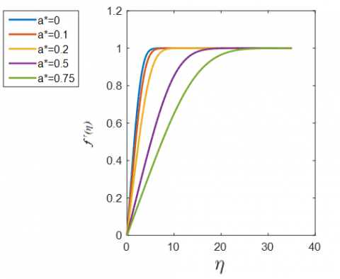
Figure 7. Velocity profile f ʹ(η) for different values of a* and x*=0, 0.5, 1
Figure 8. Shear stress f ʹʹ (η) for different values of a* and x*=0, 0.5, 1
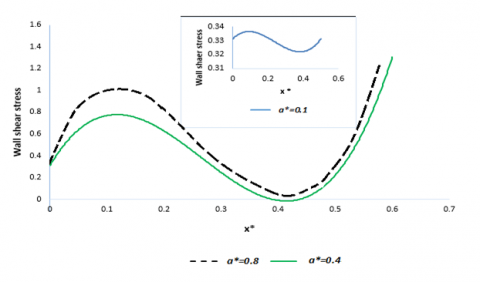
Figure 9. Wall shear stress for different values of a* and x*
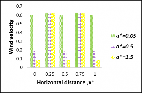
Figure 10. Wind velocity versus x* for different values of a*where Hhub=100, R=10, $u_∞=5$ and Rex= 4*105
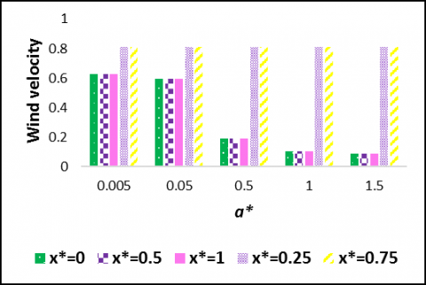
Figure 11. Wind velocity versus a* for different values of x* where Hhub=100, R=10, $u_∞=5$
Figure 12. Wind velocity for different values of Rex and $u_∞$, where Hhub=100, R=10, x*=0.5 and a*=0.5
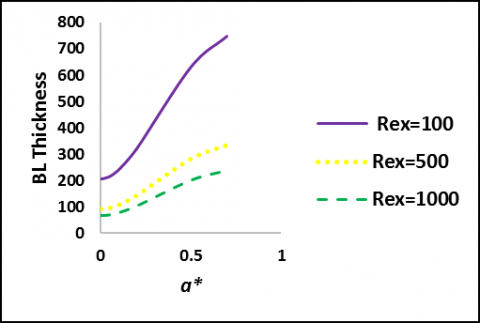
Figure 13. A representation of BL thickness based on the value of (y) at which f ʹ(η) =1
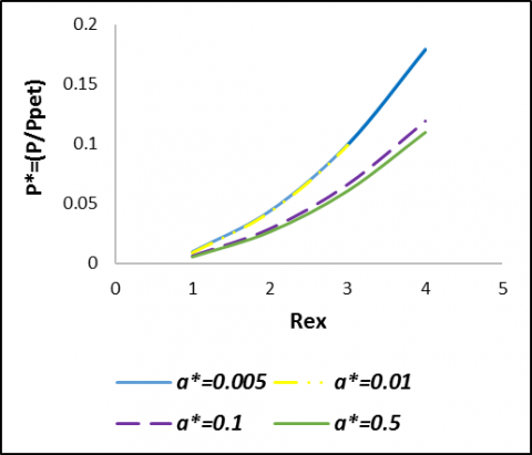
Figure 14. Wind power ratio versus wave amplitude at different Reynolds numbers
Figure 15. Wind power ratio against different turbine heights and Rex at a*= 0.1
Figure 16. Power ratio versus height for the different amplitudes (a*=1.7, 0.9, and 0.01) with Rex =4*105
Figure 17. Power ratio versus radius of wind turbine blades for the following amplitueds (a*= 0.5, 1.5)
Figure 18. Power ratio versus Tip-Speed-ratio at different amplitudes
Figure 19. Power ratio (P/Ppet) versus Reynolds number for different wave amplitudes where x*= (0, 0.5, 1), R=10, $u_∞=1$ and Hhub=100
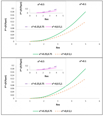
Figure 20. Power ratio (P/Ppet) versus Reynolds number for different x* and a* where R=10, $u_∞=1$ and Hhub=100
Figure 21. Wind power ratio (P/P pet) against wave amplitude for different Rex
Figure 22. Power output (P/P pet) versus amplitude for different power coefficients
Flow over a corrugated surface can affect the hydraulic characteristic of the flow through BL, it is found that the velocity decreases as amplitude values increase, since the velocity is affected slightly when a* is quite small by the roughness of the surface, and almost nothing is hindering wind speed. So, wind speed is smallest when amplitude or roughness of the surface is the most, this is due to higher shear stresses between fluid layers that comes from higher stresses at corrugated surface,
The larger the amplitude is the lesser the velocity will be; the grater the values of shear stress, stream function and wall shear stress (τ) will become. As τ reflects the tangential force extended by the flowing fluid resulted by the friction effects on the surface and between fluid layers.
As moving away from the ground, surface effect diminishes rapidly and vanishes completely outside the BL, where the flow velocity returns to the freestream velocity and becomes f ʹ(ƞ)=1. It is clear that the larger the amplitude is; the grater the BL thickness will be.
The wind power expressed based on Blasius power and Pet power, decreases when considering a corrugated surface compared to that flat one or that stream flow which propagate far away of the surface outside BL. As amplitude values getting larger, the amount of harvested power is lesser, wind power increases as the height of wind turbine increases, and decreases as the radius of wind turbine decreases.
It is found that as amplitude increases the wind velocity decreases, as a result, the wind power decreases as well as Tip-Speed-Ratio. Wind power output is grater when TSR is not so large nor so small.
It is clear that higher Rex value means high inertia forces compared to viscous forces, that in turn means that the wind velocity increases when Rex value is larger as well as wind power. It also refers to a small boundary layer thickness, which limits the viscous effects on fluid layer in a small region near the corrugated surface. It is also obvious that the more the value of u∞, the larger the values of wind velocity, where u∞ is calculated based on the value of Rex, x and v.
Since the power coefficient of a turbine is a measure of however efficiently the turbine converts the energy within the wind into electricity. The less efficient a turbine is the less of the kinetic energy is converted into electricity.
The following are suggestions for further investigations based on the previous work:
1) Finding the effect upon wind turbines, wind farms or wind energy generation considering turbulent conditions when Rex>5*105.
2) Studying the effect of fluctuating wind steams on the structure of wind turbine and its base.
3) Integration of corrugated surface function through calculations can be introduced by taking different functions instead of sine functions to describe shape of obstacles such as cosine functions or any combination of both.
|
A |
Swept rotor area in square meter |
m2 |
|
a* |
Amplitude-to-length ratio of the wavy surface (wave amplitude) |
Dimensionless |
|
Cp |
Power Coefficient of wind turbine |
Dimensionless |
|
Hhub |
Hub height of the wind turbine |
M |
|
P |
Wind power in watt |
W |
|
P |
Pressure anywhere in the field |
N/m2 |
|
R |
Radius of wind turbine blade |
M |
|
U, V |
Dimensionless velocity components along the (x, y) axes |
Dimensionless |
|
X, Y |
Cartesian coordinate component in the direction along and normal to the tangent of the surface |
M |
|
Ω |
Rotor speed |
Rad/s |
|
β (°) |
Pitch angle |
Degrees (°) |
|
Λ |
Characteristic length associated with the wavy surface |
M |
|
v |
Kinematic viscosity |
m2/s |
' Differentiation with respect to η
f ' First order component of f
F Zeroth order component of f
* Dimensionless quantities
[1] Hébrard E, Listowski C, Coll P, Marticorena B, Bergametti G, Määttänen A, Montmessin F, Forget F. (2012). An aerodynamic roughness length map derived from extended Martian rock abundance data. Journal of Geophysical Research Atmospheres 117: E04008. https://doi.org/10.1029/2011JE003942
[2] Desmond CJ. (2014). The consideration of forestry effects in wind energy resource assessment. https://doi.org/10.13140/RG.2.2.32022.04166.
[3] Cabezon D, Hansen KS, Barthelmie RJ. (2009). Analysis and validation of CFD wind farm models in complex terrain Wakes induced by topography and wind turbines. Proc. EWEC.
[4] István L, Csákberényi-Nagy G, Túri Z, Kapocska L, Tóth T, József Barnabás T. (2014). Analysis of factors affecting wind-energy potential in low built-up urban environments. Conference: Air and Water Components of the EnvironmentAt: Cluj-Napoca, Romania. https://doi.org/10.13140/2.1.4231.5200
[5] Sengupta TK. (1984). Turbulent boundary layer over rigid and moving wavy surfaces. Project: Drag Reduction. https://doi.org/10.13140/RG.2.2.35849.75366
[6] Cattin R, Schaffner B, Kunz S. (2006). Validation of CFD wind resource modeling in highly complex terrain. Meteotest, Fabrikstrasse 14, 3012 Bern, Switzerland, 1-10.
[7] Mohr M, Jayawardena W, Arnqvist J, Bergström H. (2014). Wind energy estimation over forest canopies using WRF model. Project: Forest wind - Wind Power in Forests II.
[8] Drew DR, Barlow JF, Lane SE. (2013). Observations of wind speed profiles over Greater London, UK, using a Doppler lidar. Journal of Wind Engineering and Industrial Aerodynamics. https://doi.org/10.1016/j.jweia.2013.07.019
[9] Segalini A, Fransson JHM, Alfredsson PH. (2013). Scaling laws in canopy flows: A wind-tunnel analysis. Boundary-Layer Meteorology 148(2). https://doi.org/10.1007/s10546-013-9813-2
[10] Okulov VL, Naumov I, Mikkelsen R, Sørensen JN. (2015). Wake effect on a uniform flow behind wind-turbine model. Journal of Physics, Conference Series 625(1). https://doi.org/10.1088/1742-6596/625/1/012011
[11] Odemark Y, Segalini A. (2014). The effects of a model forest canopy on the outputs of a wind turbine model. Journal of Physics Conference Series 555(1): 012079. https://doi.org/10.1088/1742-6596/555/1/012079
[12] Al-Abadi A, Youjin K., Ertunç. Ö, Delgado A. (2016). Turbulence impact on wind turbines: experimental investigations on a wind turbine model. Journal of Physics Conference Series 753(3). https://doi.org/10.1088/1742-6596/753/3/032046
[13] Juan A, Tameemi S. (2013). Wind energy analysis wind energy modelling. Conference: Energy Systems Modelling. https://doi.org/10.13140/2.1.3075.1047
[14] Agravat S, Manyam NVS, Mankar S, Tirumalachetty H. (2015). Theoretical study of wind turbine model with a new concept on swept area. Energy and Power Engineering 7(04): 127-134. https://doi.org/10.4236/epe.2015.74012
[15] Mitiku T, Manshahia MS. (2018). Project: Energy Harvesting: Modelling and Optimization of Renewable Energy Systems Using Computational Intelligence.
[16] Badran O, Abdulhadi E, Mamlook R. (1992). Projects: Renewable Energy Research Advanced Intelligent Systems.
[17] Incropera DW, Bergman and Lavine (2007). Fundamentals of Heat and Mass Transfer. (6st ed.), United States of America.
[18] Patel MR. (1999). Wind and solar power systems—design, analysis, and operation. Wind Engineering 30(3): 265266. https://doi.org/10.1260/030952406778606197