Ankita Sharma*![]() | Dhirendra Singh Bagri
| Dhirendra Singh Bagri
© 2023 IIETA. This article is published by IIETA and is licensed under the CC BY 4.0 license (http://creativecommons.org/licenses/by/4.0/).
OPEN ACCESS
Watershed dynamics are governed by geomorphic indices, which include both surface and subsurface characteristics. In this study, several hydrological indices investigate the dynamics of the Asan watershed in Uttarakhand, India focusing on the interplay between human activities and natural processes using geomorphic indices and remote sensing techniques. The research aims to achieve a planned sustainable development by understanding various geo-environmental aspects related to stream network analysis, evaluation of different terrain attributes and land-use patterns. Utilizing the use of high-resolution satellite data, such as DEM and satellite images, enhances the impact on land surface management and strengthens the overall research. The Asan watershed, designated as the 6th ordered dendritic network, exhibits the dominance of moderately permeable strata with significant discharge potential and a tectonic tilt that favours fluvial erosion. Structural influence is observed to be more pronounced in longitudinal profiles of various higher-order streams. The research shed light on rapid industrialization and urbanisation. Through the generation of decadal LULC maps from 1980 to 2016, the study reveals a four-fold increase in the urban area over the last four decades. Economic, topographic, and commercial factors contribute to these dynamic changes, which alarmed environmental scientists and planners for effective management and development.
geomorphic indices, terrain attributes, DEM, LULC, watershed
Understanding watershed dynamics and the application of geomorphic indices and GIS in watershed management play crucial roles in ensuring sustainable water resources and environmental conservation. By comprehending the intricate interactions between landforms, hydrology, and human activities within a watershed, researchers can make informed decisions for effective water management, erosion control, and flood mitigation, assess the health of watersheds, identify vulnerable areas, and implement targeted interventions, fostering a more resilient and ecologically balanced watershed management approach.
The present paper describes the drainage and terrain characteristic of the Asan watershed obtained through Remote Sensing and a GIS-based approach. Entire geomorphic and hydrologic processes that occur within the watershed contain significant information about their formation and development [1]. Geomorphic indices are responsible for providing a numerical measure of the stream network, which is an important aspect in determining a watershed’s characterization [2, 3] was the first to use quantitative techniques (mathematical equations for indices) in morphometric analysis of drainage basins from a topographic map using manual methods. Later, certain modifications in related equations were adopted by the studies [4-7].
GIS techniques are currently used for the extraction of stream networks and characterization of the watershed by several researchers [8-10]. Also, this technique helps assess various terrain attributes through the generation and study of Slope, Aspect and LULC analysis [10-12].
Several researchers have studied morphometric properties for different terrains as an indicator of structural influences on stream development [13-17]. The morphometric and morphotectonic properties have proven to be an important tool in the generation of up-to-date and statistical information for drainage basin characterization [10]. The geomorphological setup is strongly affected by the deformational processes that occur within the watershed. It is strongly dependent upon the tectonic activities occurring in it, which influences the drainage system, terrain topography and landscape development.
Many researchers studied the interplay between the structure of the drainage system and other factors such as basin relief, geology and climatic conditions present in the watershed [4, 18, 19]. In structurally active regions, the drainage network is susceptible to tectonic features such as faults, thrusts and folds, as well as tectonic movements caused by incision, diversion, tilting and asymmetry [11]. Watersheds behave as the basic unit of the riverine formations and act as an ideal entity for understanding the tectonic activity in the area [2].
Numerous studies have examined the influence of Land Use and Land Cover (LULC) on land use dynamics [20] analysed LULC changes and drivers in the Gubalafto district, North-eastern Ethiopia, over 30 years using RS, GIS, and community surveys. Cultivated and settlement areas increased by 9% while grazing land and forest cover were drastically reduced due to population growth, land insecurity, poverty, and climate change. Ensuring the sustainable utilization of resources is crucial for safeguarding the ecosystem services of the region. The study [21] employs a research approach that integrates map interpretation, RS and GIS. The study identifies the expansion of urban residential areas and evolving economic dynamics as primary drivers of changes in land use/cover, ultimately resulting in landscape degradation. Furthermore, these alterations in and around Conakry city and its adjacent urban areas over 59 years have prompted concern within both the Guinean government and the scientific community. Socio-economic development, climatic patterns, topography manipulation, and policy implementation are the key factors affecting land use/cover. [5], highlight the significance of digital change detection techniques for understanding expansion in the area. The study used RS and GIS to assess land use/land cover dynamics in Ramnagar town, Uttarakhand, over two decades (1990-2010). The built-up area and sand bar increased by 8.88% and 3.98%, while vegetation, agricultural land, and water bodies decreased by 9.41%, 0.69%, and 2.76%, respectively. The expansion was mainly towards the southern direction along National Highway-121.
All of these parameters are further validated using field visits, toposheets, aerial photographs and satellite images.
Here, this multidisciplinary study demonstrates the interplay between human activities and natural processes. By adopting an integrated approach, the study advocates for sustainable practices that encompass biodiversity & environment conservation. This involves striking a balance between the demands of the growing population, fostering economic development and implementing enhanced environmental management practices. This understanding can be extrapolated to other watersheds, providing valuable insights for studying and managing watersheds worldwide.
This research aims to examine a detailed study of different geo-environmental aspects which influenced the study area in the long run. Further, these aspects have been categorized into three specific objectives: (a) Conducting a detailed examination of geomorphic indices, which includes evaluating morphometric and morphotectonic parameters. This analysis is based on an in-depth study of the drainage network. (b) Focus on the structural impact of the watershed (c) Generation of decadal LULC maps through different satellite datasets. These maps will serve as a crucial tool for studying changes over time.
The soul of the paper lies in the integrated parametric evaluation to understand the physiography and geometry of the watershed, which is associated with the study of its formation, development, structural imbalances and geomorphic processes. Further, the generation of LULC maps for different years helps us to study the historical and present condition of the watershed which leads to the rapid expansion of built-up areas over time compared to the forest and agricultural land.
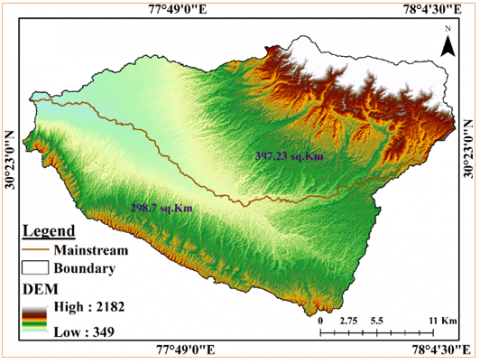
The Asan River watershed is situated in the Dehradun district, Uttarakhand state, India (Figure 1). Asan River is the perennial tributary of the Yamuna River that flows northwest of Doon Valley and eventually joins them at Dhalipur (a small hamlet in Vikasnagar). It extends from geographic latitudes 30° 14' 14'' N to 30° 29' 54'' N and longitudes 77° 39' 42'' E to 78° 05' 30'' E. The outlet of the watershed has a minimum elevation of 349m present in the western direction of the watershed while the Lesser Himalayan range present in the northern direction of the watershed has an elevation of 2182m above mean sea level (MSL). It falls under the 53F/11, 53F/15, 53J/3 and 53F/16 toposheet of Survey of India, scale (RF)-1: 50,000.
Figure 1. Location map of the study area and DEM used
2.1 Watershed’s characteristics
The watershed seems to have a temperate climate. Depending on the elevation of the area, this can range from tropical to cold and rainy. Also, because the watershed is surrounded by hilly terrain, temperature fluctuations due to elevation differences are significant [22]. The Siwalik hills (about 800m) have a sub-tropical climate whereas the areas with an elevation of 800m-2400m have a temperate climate [23]. Due to the unique physiography of the watershed, the movement of monsoon wind is significantly hampered, leading to distinctive rainfall patterns. Approximately 85% of the total annual rainfall is concentrated during the summer months. This brings much-needed water to the plains and its percolation into the rocks and replenishes the water table. Summer is pleasant in the hilly regions, though not to the same extent as in the plains of the adjacent district. The annual average rainfall over the watershed ranges from 1274mm to 1766.7mm. The watershed receives the majority of its annual rainfall from June to September, with July and August being the wettest months [24, 25]. The monthly statistics reveal that the mean temperature of the study area ranges from 12.04°C (minimum) for January to 28.9°C (maximum) for June with an annual average temperature is 21.90°C [24]. The total area and perimeter of the watershed are 695.9Km2 and 180.4Km respectively.
At the foothills of the Siwalik ranges, the Asan River forms one of the most prominent watersheds in Doon Valley, flowing northeast to southwest through the central portion of the valley. The length and width of the Asan watershed are approximately 40Km and 18Km respectively. The Asan Barrage is located in the vicinity of rivers Asan and Yamuna. The Asan River serves as the tributary of the Yamuna River flowing northwest through the Doon Valley and later joins the Yamuna River in Dhalipur village at Vikasnagar. It is a perennial river and the origin is from Chandrbani (spring water) in the Dehradun district. The watershed is covered with a thick pile of Doon gravel which serves as a good unconfined aquifer. These aquifers may be responsible for fulfilling the basic domestic and irrigation. Also, their contribution increases at the higher reaches of the watershed because of precipitation requirements [26]. But the continuous extraction, if exceeds recharge, of this source leads to its depletion and may deteriorate water quality as the concentration of salts increases [27]. The soil belonging to Siwalik is sandy loam with bands of clay, along with conglomerate and sandstone, which give cohesion to the soil and thus enhance its physical characteristics.
The soil is shallow and dry in the upper reaches of the watershed compared to the lower slope, this results in the dominance of xerophytic vegetation at higher elevations [28]. Soil with a good proportion of clay creates adequate drainage in the lower reach. In this unit, groundwater is found in both confined and unconfined conditions.
2.2 Physiographic characteristics
The physiographical feature of the watershed is the sharp rise in the Lesser Himalayan range, locally known as Mussoorie Hill in the north and Siwalik in the south. The Asan is a stream-fed river having an approximate length of 43Km. The river flows through the Bijapur Canal following the Tapkeshwar Mahadev Shrine. As the river proceeds towards the southwest, it carries water from several streams flowing southward from the Lesser Himalayan range and northward from Siwaliks. At the lower reaches, it flows a relatively flat section that feeds the Asan barrage. It is located in the vicinity of rivers Asan and Yamuna. The water from the barrage later drains into the Yamuna at Paonta Sahib (Figure 2).
Figure 2. Landscape view of the Asan Conservation Reserve
The soil type in the watershed varies from the alluvial soil of the Terai belt to the recent alluvium of the Doon, the fragile soil of Siwalik, bare soils [23].
In India, this convection struck on February 1, 1982. India currently has 42 wetlands, the most in South Asia. The Asan Barrage dammed the river in 1967, resulting in siltation above the dam wall, which aided in the creation of bird-friendly habitats. It has been adopted as the 38th Ramsar site in India on 21st ‘July’ 2020 (Figure 2). The critically endangered white-rumped vulture (Gyps bengalensis), red-headed vulture (Sarcogyps calvus), red-crested pochard (Netta rufina), Baer's pochard (Aythya baeri), ruddy shelduck (Tadorna ferruginea) are among the significant species found here. There are different fish species, including the endangered Putitor mah. They remain, however, one of the world's most endangered ecosystems, owing to ongoing pollution, drainage, and resource overexploitation.
2.3 Socio-economic characteristics
The socio-economic structure of rural communities in the watershed is defined by a simple subsistence economy mainly focused on self-consumption. Furthermore, the people rely on rain-fed agriculture. Continuous physical labour, cultivation practice on gentle slopes (central part of the watershed), as well as moderate to steep slopes (mountainous terrain), fetching fodder, fibrous grasses, fuelwood and delivering products to the market, are all necessary for survival. The watershed has good road connectivity for all livelihood needs and services. Rain-fed areas are often agro-forestry zones, with grasses, bushes, trees and livestock all contributing to the overall system [23]. In the Lesser Himalayan zone, however, agriculture is practised in the form of terrace farming on moderate to steep slopes (Figure 3(c)). Controlling water movement, runoff, soil erosion and maximizing water penetration are some of the responsibilities of this practice. Agriculture is the second-largest class in terms of area covered, after the forest (Table 1). The majority of the trees in this area are double-cropped. Even though water scarcity is a major issue in this region, farmers try to grow crops during both the Rabi and Kharif seasons. The mixed forests are dominated by trees that cover more than 60% of the area and grow to a height of more than 2m. The forest covers nearly 410Km2 (~57%) of the total area of the watershed.
Figure 3. Different features in the watershed impacting the socio-economic activities
Table 1. Classified area under different LULC categories for 1980, 1995, 2008 and 2016 in the study area
|
|
1980 |
1995 |
2008 |
2016 |
||||
|
LULC/Class |
Area (Km2) |
Area (%) |
Area (Km2) |
Area (%) |
Area (Km2) |
Area (%) |
Area (Km2) |
Area (%) |
|
Built-up |
9.13 |
1.31 |
11.71 |
1.68 |
24.43 |
3.51 |
35.50 |
5.10 |
|
Cropland |
202.02 |
29.03 |
199.68 |
28.69 |
196.76 |
28.27 |
193.71 |
27.84 |
|
Fallow land |
13.24 |
1.90 |
13.24 |
1.90 |
11.49 |
1.65 |
11.49 |
1.65 |
|
Plantation |
22.45 |
3.23 |
22.41 |
3.22 |
21.14 |
3.04 |
14.81 |
2.13 |
|
Evergreen |
54.14 |
7.78 |
54.14 |
7.78 |
53.49 |
7.69 |
53.24 |
7.65 |
|
Deciduous |
335.26 |
48.18 |
334.95 |
48.13 |
335.99 |
48.28 |
335.93 |
48.27 |
|
Mixed |
5.53 |
0.79 |
5.53 |
0.79 |
5.53 |
0.79 |
5.53 |
0.79 |
|
Waterbodies |
54.15 |
7.78 |
54.27 |
7.80 |
47.10 |
6.77 |
45.72 |
6.57 |
|
|
695.92 |
100.00 |
695.92 |
100.00 |
695.92 |
100.00 |
695.92 |
100.00 |
Table 2. Geographic location of spring’s distribution over the study area
|
Number |
Latitude |
Longitude |
Number |
Latitude |
Longitude |
|
1. |
30.42 |
77.90 |
24. |
30.37 |
77.97 |
|
2. |
30.46 |
77.90 |
25. |
30.37 |
77.94 |
|
3. |
30.48 |
77.86 |
26. |
30.38 |
77.79 |
|
4. |
30.42 |
77.75 |
27. |
30.39 |
77.78 |
|
5. |
30.42 |
77.75 |
28. |
30.39 |
77.88 |
|
6. |
30.36 |
77.71 |
29. |
30.39 |
77.91 |
|
7. |
30.34 |
77.72 |
30. |
30.40 |
77.94 |
|
8. |
30.34 |
77.73 |
31. |
30.40 |
77.94 |
|
9. |
30.34 |
77.75 |
32. |
30.41 |
77.96 |
|
10. |
30.28 |
77.92 |
33. |
30.39 |
77.97 |
|
11. |
30.29 |
77.90 |
34. |
30.39 |
77.97 |
|
12. |
30.29 |
77.97 |
35. |
30.40 |
77.98 |
|
13. |
30.37 |
77.99 |
36. |
30.39 |
77.99 |
|
14. |
30.46 |
77.98 |
37. |
30.40 |
77.99 |
|
15. |
30.42 |
77.94 |
38. |
30.43 |
77.98 |
|
16. |
30.42 |
77.95 |
39. |
30.45 |
78.05 |
|
17. |
30.39 |
77.95 |
40. |
30.44 |
78.06 |
|
18 |
30.40 |
77.95 |
41. |
30.40 |
78.03 |
|
19. |
30.39 |
77.95 |
42. |
30.41 |
78.06 |
|
20. |
30.38 |
77.96 |
43. |
30.42 |
78.08 |
|
21. |
30.38 |
77.96 |
44. |
30.45 |
78.07 |
|
22. |
30.37 |
77.96 |
45. |
30.46 |
78.02 |
|
23. |
30.38 |
77.96 |
|
|
|
Figure 4. Distribution of spring in the watershed
The majority of them are classified as reserved/protected areas. Many mountainous streams can be found in the higher reaches, which are used to provide an abundance of water throughout the year. Water for domestic use is still sourced from springs, tap springs, ground seeps flowing through mountain streams, or rainwater harvesting structures (Figure 3(d)). The distribution of springs with their geographic locations in the study area is shown in Figure 4 and Table 2.
However, streams and springs are drying up and the hydrological pattern in mountainous areas is shifting. This is due to population growth and anthropogenic activities but residents are causing damage to mountainous hydrological systems (Figure 3(a)). Different physical processes such as deforestation, siltation, mass wasting etc., influence the hydrology of the area predominantly at different scales [29].
Asan River flows along the axis of the asymmetrical synclinal valley. It arises in the clayey dipping in the west of the Asarori-Dehra Road and afterwards the northwesterly course of about 42 Km, it merges into the Yamuna. The physiographic units of the watershed are striking in NW-SE to ENE-WSW. The research area is located in the Doon valley. The watershed lies between Lesser/Lower Himalaya to the north and the Outer Himalaya (Siwalik) to the south. The northern and southern part of the watershed is characterized by rough mountainous terrain having rocks predominantly of sedimentary and metamorphic origin. Small seasonal channels from the Siwaliks and Mussoorie that meet the mainstream are almost dry for the majority of the year. The drainage pattern is influenced by slope, lithology and structure to determine the severity of erosion. It is also susceptible to tectonic features viz., faults, folding and tilting. The major portion of the study area is covered by a piedmont zone containing pebbles, gravels, boulders etc., with scanty exposures of Siwalik in the southern part of the watershed. These have been transverse by several structural dislocations, namely the Main Boundary Fault (MBF), exposed in the north along with other associated lineaments, some of which are tectonically active. The entire watershed is divided into four major hydrogeological/lithostratigraphic units viz., Lesser Himalaya, Siwaliks, Doon gravels and recent alluvium. Stratigraphically, each succession is the representation of age, thickness and environment of deposition [30, 31]. Their stratigraphic description is mentioned in the subsequent sections (Figure 5, Table 3).
The directional alignment of structural features such as faults and thrusts from NE to SW through the north-western part of the Doon Valley. The study area is bounded in the north by the Main Boundary Thrust (MBT) with the Lesser Himalaya and in the south by the Mohand Thrust with the Lower Siwalik, which falls outside the watershed. The MBT situated in the region brings Lesser Himalaya (Precambrian) strata over Doon fan gravel (Quaternary). The activities of various faults and thrusts provide maximum relief into the watershed [32]. The Santaugarh thrust [33, 34], the Bhauwala thrust [35], the Asan and Tons Faults [36], are the other structural features present in the area. The MBT and rocks of Middle Siwalik ride over the older fan deposits whereas the younger fan deposits are eroded into the Santaugarh Fault hanging blocks. This indicates that the fan gravel found in the area is derived from the erosion of MBT and Santaugarh hanging blocks.
Figure 5. Geological and structural map of the Asan watershed [30, 34]
The foothills of the previously mapped Mussoorie hills descend in a number of large fans made up of pebbles, cobbles, and boulders with a sandy matrix [37]. An alluvial fan is formed by the accumulation of sand, gravel, silt, etc. (collectively known as alluvium) over a long period due to the interaction of the river of the stream with mountains or hills. Because of their resemblance with a fan or section of a shallow cone, it is called an alluvial fan. It is one of the major geomorphological units of the watershed identified by the studies [32, 36]. The maximum and minimum elevation of the Alluvial fan ranges from 1778m to 345m above MSL and covers an area of 133.51Km2~18.74% of the entire watershed and the slope ranges from <5° i.e., gentle. The three alluvial fans Donga, Dehradun, and Bhogpur flow from west to east through the Lesser Himalaya's front range, depositing terraces made of a loose mixture of gravel, sand, silt, and clay along the Asan, Song, and Tons rivers. In addition, a system of springs covers the entire area [31]. Both the northern and southern portions have rugged mountainous terrain, with the majority of the rocks being sedimentary and metamorphic in origin.
Table 3. Lithostratigraphic succession of Doon Valley [30, 35]
|
Age |
Geological Units/Formations |
Description of Lithology |
|
|
Recent |
River alluvium |
Lenticular, elongated and medium to fine, unconsolidated sand, Silt and clay generally belong from Upper Siwalik |
|
|
Late Pleistocene to Early Holocene |
Doon fan gravel |
Boulders, pebbles, sand, quartzite and clay generally belongs to Lesser Himalayan and Siwalik |
|
|
Late Pleistocene |
Old Doon gravels |
Rounded boulders, pebbles, sand and clay |
|
|
UNCONFORMITY |
|||
|
Late Pliocene to Early Pleistocene |
Upper Siwalik |
Conglomerate, coarse boulders and clay bed |
|
|
Late Miocene to Early Pliocene |
Middle Siwalik |
Micaceous and intercalation of clay, sandstone |
|
|
Middle Miocene |
Lower Siwalik |
Compact sandstone silt and interbedded clay and shale intercalations |
|
|
UNCONFORMITY/Main Boundary Thrust |
|||
|
Palaeocene to Early Eocene |
Subathu Formation |
Red Shale, limestone and lenticular sandstone |
|
|
UNCONFORMITY/Krol Thrust |
|||
|
Proterozoic |
Krol |
Krol E |
Dolomitic limestone and Shale |
|
Krol D |
Dolomitic limestone |
||
|
Krol C |
Limestone with massive sulphurous content |
||
|
Krol B |
Shale |
||
|
Krol A |
Limestone |
||
|
|
Infra-Krol/Blaini |
Dark shale, slate, boulder beds and quartzite, dolomite |
|
|
Nagthat |
Quartzite, slate shale |
||
|
Chandpur |
Phyllite, quartzite, slate, limestone with the presence of quartz bands |
||
Significant information about the characteristics of the streams and watershed behaviour has been extracted from quantitative analysis of the stream network. In tectonic geomorphology, the Digital Elevation Model (DEM) is used for better analysis of topographic parameters and database generation. Details of the data used in the present study are shown in Table 4. Further, HEC-GeoHMS extension in ArcGIS v. 10.3 software is used to delineate the watershed, extraction of drainage channels and evaluation of different indices are explained in Tables 5 and 6.
The following methodological procedure is adopted for the accomplishment of the present work:
Using the WGS 84 datum and UTM projection, the toposheets are geometrically rectified and georeferenced through ground control points (GCPs). In addition, ERDAS Imagine 9.1 image processing software is used to mosaic all geocoded toposheets.
The drainage network of the watershed is generated through the following geo-processing techniques: ALOS-PALSAR > Filled DEM > Flow direction > Flow accumulation > Stream network generation > Watershed Extraction. The DEM used in the study is depicted in Figure 1.
The geomorphic indices are assessed by using the morphometric and morphotectonic approaches. Thereafter, the results are determined through a quantitative parametric analysis using the standard mathematical equations shown in Tables 5 and 6.
Through digitizing different feature classes from the subsequent satellite images, four decadal LULC maps of the area are created (Figure 6). The relevant details about the satellite images are shown in Table 4. Thereafter, calculating the area covered by each feature class, we concluded that, by contrasting the earlier and more recent scenarios within the region (Table 1).
Figure 6. Land use land cover map of the study area [22]
Table 4. Detailed information of dataset used for the present study
|
Data |
Details |
Sources |
||||
|
Toposheets |
53F/11, 53F/15, 53F/16 & 53J/3 (RF*-1:50,000) |
Survey of India (SOI), Dehradun, India |
||||
|
ALOS-PALSAR* |
Spatial Resolution-12.5m |
EORC*/JAXA* |
||||
|
Data description used for LULC classification |
||||||
|
Reference year |
Data/Sensor |
Path-Row |
Number of Bands |
Spatial Resolution |
Date of Acquisition |
Sources |
|
1980 |
Landsat 3 MSS* |
Path-157 Row-039 |
4 |
60m |
19/03/1980 |
USGS* |
|
1995 |
Landsat 5 TM* |
Path-146 Row-039 |
7 |
30m |
06/12/1995 |
|
|
2008 |
Landsat 5 TM* |
Path-146 Row-039 |
7 |
30m |
03/04/2008 |
|
|
All the images of Landsat have a scene size of approximately 170km north-south by 185 km east-west. |
||||||
|
2016 |
Resourcesat-2 LISS-IV* |
Path-96 Row-49 |
3 |
5.8m |
08/04/2016 |
NRSC* ISRO* |
|
Path-96 Row-49 |
02/05/2016 |
|||||
|
Path-96 Row-50 |
08/04/2016 |
|||||
|
Path-96 Row-50 |
02/05/2016 |
RF*=Representative Fraction
ALOS-PALSAR*=Advanced Land Observing Satellite-Phased Array type L-band Synthetic Aperture Radar
EORC*=Earth Observation Research Centre
JAXA*=Japan Aerospace Exploration Agency
MSS*= Multispectral Scanner
TM*= Thematic Mapper
USGS*=United States Geological Survey
LISS*=Linear Imaging Self Scanning Sensor
NRSC*=National Remote Sensing Centre
ISRO*=Indian Space Research Organisation
Table 5. Detailed methodology of geomorphic indices related to the morphometric analysis
|
No. |
Parameters |
Formula |
Explanation |
Reference |
|
1. |
Stream Order (Su) |
The hierarchical rank of tributaries |
- |
Strahler 1964 |
|
2. |
Number of Stream of each order (Nu) |
Total number of streams of a given order |
- |
Strahler 1952 |
|
3. |
Stream Length (Lu) |
Total Length of the streams |
- |
Horton 1945 |
|
4. |
Length of mainstream (Lum) |
Length of the highest order stream |
- |
- |
|
5. |
Mean stream length (Lum) |
$\begin{gathered}\boldsymbol{L}_{\boldsymbol{u m}}=\boldsymbol{L}_{\boldsymbol{u}} / \boldsymbol{N}_{\boldsymbol{u}} \\ \boldsymbol{L}_{\boldsymbol{u}}=\text { Total Stream length of ' } S_u \text { ' order } \\ \boldsymbol{N}_{\boldsymbol{u}}=\text { Total number of stream segments } \text { of order ' } S_u \text { ' }\end{gathered}$ |
- |
Strahler 1952 |
|
6. |
Stream length ratio (Lur) |
$L_{u r}=L_u / L_{u-1}$ $\boldsymbol{L}_{\boldsymbol{u}}=$ Total stream length of stream order ' $S_u$ ' $\boldsymbol{L}_{u-1}=$ Total stream length of its next lower order |
- |
Horton 1945 |
|
7. |
Bifurcation ratio (Rb) |
$R_b=N_u / N_u+1$ $\boldsymbol{N}_{\boldsymbol{u}}=$ Total number of stream segments of order ' $S_u$ ' $\boldsymbol{N}_{\boldsymbol{u}}+\mathbf{1}=$ Number of stream segment of next higher order |
≥ 4: Higher ‘ $R_b$ ’/younger stage 3.5-4: Moderate ‘ $R_b$ ’/mature stage ≤3.5: Lower ‘$R_b$’/ older stage |
Strahler 1964 |
|
8. |
Mean Bifurcation Ratio (Rbm) |
Average of bifurcation ratio of all orders |
<3: Flat region 3-5: Least effect of geological structure on the drainage pattern >5: Structurally controlled |
Strahler 1964 |
|
9. |
Perimeter (P) |
GIS software analysis |
- |
Schumm 1956 |
|
10. |
Basin Length (Lb) |
The longest dimension of the watershed |
- |
Schumm 1956 |
|
11. |
Area (A) |
GIS software analysis |
- |
Schumm 1956 |
|
12. |
Drainage Density (Dd) |
$D_d=\Sigma L_u / A$ $L_u$ = Stream Length A=Area |
0-1: Low 1-2: Moderate 2-3: Moderately high 3-4: High 4-5: Very high |
Horton 1932 1945 |
|
13. |
Stream Frequency (Fs) |
$F_s=\Sigma N_u / A$ $N_u$ =Total number of stream of all orders A=Area of watershed |
0-1: Low 1-2: Moderate 2-3: Moderately high 3-4: High 4-5: Very high |
Horton 1932 1945 |
|
14. |
Drainage Texture (Dt) |
$D_t=\Sigma N_u / P$ $N_u$ =Total number of stream of all orders P=Perimeter |
<2: Very Coarse 2-4: Coarse 4-6: Moderate 6-8: Fine >8: Very Fine |
Smith 1939 |
|
15. |
Length of overland flow (Lg) |
$L_g=1 / D_d * 2$ $D_d$ =Drainage density |
<0.2: Low flow path 0.2-0.3: Moderate flow path >0.3: High flow path |
Horton 1945 |
|
16. |
Elongation ratio (Re) |
$\boldsymbol{R}_{\boldsymbol{e}}=\mathbf{2}(\sqrt{\mathbf{A} / \pi}) / \boldsymbol{L}_b$ A=Area of watershed $L_b$ =Basin length π=3.14 |
<0.7: Elongated 0.7-0.8: Less elongated 0.8-0.9: Oval 0.9-1.0: Circular |
Schumm 1956 |
|
17. |
Basin Relief (H) |
H=Z-z Z=Maximum Height of the basin z=Height of Basin Mouth |
- |
Strahler 1952 |
|
18. |
Relief Ratio/ Watershed Slope (Rh) |
$\boldsymbol{R}_h=\boldsymbol{H} / \boldsymbol{L}_b$ H= Basin Relief $L_b$ =Basin Length |
≥0.29: Steep 0.28-0.17: Moderate <0.17: Gentle |
Schumn 1956 |
|
19. |
Ruggedness Number (Rn) |
$R_n=D_d *(H / \mathbf{1 0 0 0})$ H=Basin Relief $D_d$=Drainage Density |
<1: Low 1-2: Moderately low 2-3: Moderate 3-4: Moderately high >4: High |
Strahler 1968 |
Table 6. Detailed methodology of geomorphic indices related to the morphotectonic analysis
|
Morphotectonic Parameters |
||||
|
No. |
Parameters |
Formula |
Explanation |
References |
|
1. |
Drainage Basin Asymmetry (Af) |
$A_f=100\left(A_r / A_t\right)$ $A_r$ =Area of the right (facing downstream) of the mainstream $A_t$ =Area of the watershed |
$A_f$=50: Stable environmental setting $A_f$>50: Tilting suggested to the left side $A_f$<50: Tilting suggested to the right side |
Molin 2004 |
|
2. |
Channel Sinuosity Index (CSI) |
$C_{S I}=C_l / V_l$ $C_{S I}$ =Channel Sinuosity Index $C_l$ =Channel Length $V_l$ =Valley distance |
$C_{S I}$ <1.05: Almost Straight $C_{S I}$ >1.05: Sinuous $C_{S I}$ >1.50: Meandering $C_{S I}$ >1.3: Braided $C_{S I}$ >2.0: Anastomosing |
Mueller 1968 |
|
3. |
Basin shape Index (Bs) |
$\boldsymbol{B}_s=\boldsymbol{L}_b / \boldsymbol{W}_b$ $L_b$ = Length of a watershed measured from the headwaters to the mouth, $W_b$ = Width of the watershed at its widest point |
$\boldsymbol{B}_s$ =1.7-3.22 (Elongated basin) $\boldsymbol{B}_s$ =1.21-1.76 (Semi-elongated basin) $\boldsymbol{B}_s$ =1.11-1.20 (Circular basin) |
Mahmood & Gloaguen 2012 |
|
4. |
Stream Length Gradient Index (SLindex) |
$S L_{\text {index }}=(\Delta H / \Delta L) L$ ∆H= Variation in altitude ∆L=Length of a reach L= Horizontal length from the watershed divide to a midpoint of the reach |
$S L_{index }$≤500: Tectonically active area $S L_{index }$=300-500: Moderately active $S L_{index }$<300: Least active |
Hack 1973 |
|
5. |
Hypsometric Integral (Hi) |
$H_i=\left(E_{\text {mean }}-E_{\text {min }}\right) /\left(E_{\text {max }}-E_{\text {min }}\right)$ $E_{mean}$=Mean elevation value $E_{max}$= Maximum elevation value $E_{min}$= Minimum elevation value (outlet) |
$H_i$≤0.3: Old stage; maximum stability, low erosional susceptibility 0.3≤$H_i$≤0.6: Mature stage; moderate erosional susceptibility $H_i$≥0.6: Young stage; high erosional susceptibility |
Strahler 1952 |
The current study is based on the evaluation of various parameters which are assessed by incorporating information from topographic maps, satellite datasets which include images and the DEM along with the different mathematical equations listed in Tables 5 and 6. These are useful in determining the significant knowledge regarding the presence and identifying the location of geological structures like faults and thrusts, differential uplift, erosional control, and the distribution of tectonism in the region. Based on an analysis of the drainage network and its characteristics, this study evaluates 19 morphometric parameters and 5 morphotectonic parameters individually. Furthermore, a quantitative approach to determining the structural impact in the watershed is also focused, in addition to morphological characteristics.
The Main Boundary Thrust, Santaugarh Thrust, Mahajaun Thrust, Bhauwala Thrust, Nun River Fault, and Asan Fault are some of the significant structural features of the watershed's stretch. Tons Fault and Asan Fault are located in the central and northern portions of the study area, respectively.
The slope and aspect map capture both the direction of slopes (aspect) and their steepness (degree) respectively. The LULC classification, areal description and the analysis of the present status of different classes of the watershed are carried out for the research in subsequent sections:
5.1 Morphometric analysis
The morphometry of watersheds is the “measurement of surficial features formed due to endogenetic as well as exogenetic processes” [38]. Several parameters related to the morphometric analysis with mathematical equations is shown in Table 5.
5.1.1 Linear aspect of drainage pattern & channel network
Linear aspects are closely related to the analysis of the topographical characteristics of the stream network. The linear aspect gives information about the unidimensional features of the watershed. The mathematical equations associated with the parameters are described in Table 5.
The stream network of the Asan watershed extends to the sixth-order for the variable threshold of 0.18 Km2 or 1200 cells and shows the dendritic and trellis type of stream network which is an indication of texture’s homogeneity (Figure 7). This pattern emerges when the river channel follows the terrain’s slope and lithology must be impermeable and non-porous [39]. The number of streams ($N_u$) belongs to their respective order are determined and it is shown in Table 7. It’s worth noting that the first-order has the highest number of 805 streams, while the stream frequency decreases as stream order increases, with the sixth-order having the lowest i.e., 1. The sum of streams for each order gives its stream length ($L_u$). Table 7, shows that the sum of ‘$L_u$’ is dominant for first-order streams (745 Km). From the first order to the successive higher order, the sum of stream length is observed to decrease.
The study [40] defines Bifurcation ratio ($R_b$) as “the ratio between the total number of streams ($N_u$) and the number of streams of the next higher-order ($N_u$+1)”. The value of the ‘$R_b$’ for the watershed ranges from 3-5 for all orders. The drainage network with high '$R_b$' indicates that the area is tectonically active with prominent soil erosion [2]. Higher ‘$R_b$’ represent the younger stage while the lower value indicates the mature stage of development [41]. The mainstream (Asan River) passes through the Asan Fault (AF) which corresponds to higher ‘$R_b$’ (Figure 5). This supports that mainstream formation is younger than the geologic structures. Mean Bifurcation Ratio ($R_{bm}$) for the watershed is 3.9.
Table 7. Tabular classification representing characteristics of streams
|
ALOS- PALSAR |
$S_u$ |
$N_u$ |
$L_u$ (Km) |
$L_{um}$ |
$L_{ur}$ |
$R_b$ |
$R_{bm}$ |
|
1 |
805 |
745 |
0.9 |
- |
- |
|
|
|
2 |
258 |
502 |
1.9 |
2.1 |
3.1 |
|
|
|
3 |
67 |
274 |
4.1 |
2.1 |
3.9 |
|
|
|
4 |
20 |
137 |
6.9 |
1.7 |
3.4 |
|
|
|
5 |
15 |
39 |
7.8 |
1.1 |
4.0 |
|
|
|
6 |
1 |
43 |
43.0 |
5.5 |
5.0 |
|
|
|
Total |
|
1156 |
1740 |
64.6 |
12.5 |
19.3 |
3.9 |
$\boldsymbol{S}_{\boldsymbol{u}}:$ Stream order, $\boldsymbol{N}_{\boldsymbol{u}}:$ Number of streams, $\boldsymbol{L}_{\boldsymbol{u}}:$ Stream Length, $\boldsymbol{L}_{u m}:$ Mean stream length, $L_{u r}:$ Stream length ratio, $\boldsymbol{R}_b:$ Bifurcation ratio, $\boldsymbol{R}_{b m}:$ Mean Bifurcation ratio
Figure 7. Stream network belongs to different stream order of the study area
Based on the classification given by the study [42], ‘$R_{b m}$’ is classified into three categories <3: flat region; 3-5: least effect of geologic structure on drainage network; >5: drainage network is structurally controlled. The calculated value of ‘$R_{b m}$’ indicates low structural impact and the presence of moderate slopes on the drainage development of the watershed.
5.1.2 Aerial aspect of the watershed
The aerial aspects of the watershed share a significant connection with the study of two-dimensional features of the watershed. The mathematical equations associated with the parameters are described in Table 5.
The texture and proximity of channels within a watershed are predicted by drainage density $\left(D_d\right)$. Based on the classification adopted after [43], the value of ‘$D_d$’ ranges from 0 to 5 based on lower to higher degree of density; 0-1: Low, 1-2: Moderate, 2-3: Moderately high, 3-4: High, 4-5: Very high. In the present study, it is calculated as 2.1 Km-1 which indicates that the area comes within the range of medium drainage density and rock surfaces drained by the watershed having moderately permeable strata with medium run-off and infiltration [41]. Drainage texture ($D_t$) is a degree of the relative spacing of drainage lines in a fluvial-dissected terrain [6]. The calculated ‘$D_t$’ for the area is 6.32 Km. According to Smith’s classification, the different categories of ‘$D_t$’ are: <2: Very Coarse; 2-4: Coarse; 4-6: Moderate; 6-8: Fine; >8: Very fine. Based on the classification, the watershed represents moderate drainage texture. It also indicates that the area is developed on a bedrock of moderate permeability (e.g., thin-bedded sandstone). Stream frequency ($F_s$) is “the total number of stream segments of all orders per unit area” [43]. Based on the classification which categorises ‘$F_s$’ into five categories: 0-1: Low; 1-2: Moderate; 2-3: Moderately high; 3-4: High; 4-5: Very high. Using the methodology (Table 5), the calculated ‘$F_s$’ for the study area is 1.64 Km2 which indicates that the watershed has moderate ground slopes, rock permeability, run-off and infiltration capacity of the watershed [43, 44]. The length of overland flow ($L_g$) is “the length of water over the ground before it gets concentrated into certain stream channels approximately equal to half of the reciprocal of drainage density” [4]. It affects the geographical and hydrological development of the watershed. Based on the length of the flow path, ‘$L_g$’ is classified into different categories: <0.2: Low flow path; 0.2-0.3: Moderate flow path; >0.3: High flow path. The calculated value of ‘$L_g$’ is 0.24 shows a well-developed stream network with moderate slopes showing surface runoff travels at a relatively shorter distance before flowing through the channels. The horizontal projection of the watershed shape can be represented using the Elongation Ratio ($R_e$) [45]. The calculated value of ‘ $R_e$ ’is 0.47. According to the classification adopted after [40], ‘$R_e$’ is divided into different categories based on the shape of the watershed: <0.7: Elongated; 0.7-0.8: Less elongated; 0.8-0.9: Oval; 0.9-1.0: Circular. This indicates that the shape of the watershed is elongated with low to medium relief and moderate infiltration.
5.1.3 Relief aspect of the watershed
The relief aspects of the watershed share a significant connection with the “study of the three-dimensional feature includes area, volume and altitude of the vertical dimension of landform to analyses of varying geohydrological characteristics” [6]. This aspect helps in the study of various geomorphological features which includes analysis of terrain relief, computing surface, permeability, sub-surface flow, and landform development. The mathematical equations associated with the parameters are described in Table 5.
Basin Relief (H) described as “the basin relief refers to differences in elevation between the drainage summits and the watershed outlet” [6]. It is helpful to understand the processes of geomorphology and several landform characteristics. Basin Relief (H) of the watershed is 1833m, with a minimum value (z) is 349m in the vicinity of the mouth (outlet) and a maximum value (Z) of 2182m in the Lesser Himalayan region. It indicates runoff and transportation of sediments from the upper to the lower reaches of the watershed. Relief ratio ($R_h$) is “the indicative of the stream’s gradient flow and intensity of erosional process operating on the slope of the watershed” [40]. According to the classification adopted after [3], the ‘$R_h$’ is classified based on the degree of steepness of the slope present in the watershed and is categorised into several categories: >0.29: Steep; 0.28-0.17: Moderate; <0.17: Gentle. The calculated value of ‘$R_h$’ is 0.23, which indicates the dominance of moderate to gentle slopes and less resistant rocks in the watershed. Ruggedness number ($R_n$) measures the extent to which basin topography is dissected [7]. According to classification of basin ruggedness [46], the different categories include: <1: Low; 1-2: Moderately low; 2-3: Moderate; 3-4: Moderately high; >4: High. The calculated ‘$R_n$’ of the study area is 3.8 which suggests that the watershed has rugged topography and is susceptible to erosion.
5.2 Morphotectonic parameter
The purpose of the qualitative and quantitative analysis is to describe the part of tectonism that controls river behaviour and the development of drainage networks [14, 47, 48]. The entire Doon valley has experienced strong denudational forces and most of the streams in the valley transported a huge number of debris. Failure of sediments, deformed rocks, jointed and shattered rocks, and prominent landslides are all of the results of tectonism prevalent in the study area. The Doon is bordered on the east by Ganga and on the west by the Yamuna, both of the rivers are flowing along the tear fault mark. The Lesser Himalayan zone, which rises abruptly to approximately 2000m in the area, is represented by the northern portion of MBT, whereas the Siwalik hills, which rise to approximately 640m and are longitudinally transverse by the Santaugarh Fault, are represented by the southern portion of MBT [34]. A broad, active syncline runs through the heart of the Doon Valley. The MBT runs parallel to the Santaugarh and Bhauwala Thrust. Several parameters are used in the study with their mathematical equations, described in Table 6.
Figure 8. Drainage Basin symmetry
5.2.1 Basin Asymmetry Factor ($A_f$)
The Basin Asymmetry Factor ($A_f$) is “the ratio of the right side of the stream facing downstream to the total area of the watershed” [15]. This parameter determines the tilting of the watershed due to lateral tectonic shift concerning the trunk-ordered stream at smaller as well as larger scales [15, 49].
From the methodology adopted by the study [50], the calculated value of ‘$A_f$’ is 57, which suggests tilting toward the left side of the area (Table 6). In Figure 8, it is also found that the mainstream of the watershed flows towards the NE direction and tilts toward the south. The tributaries on the right side of the trunk stream cover a larger area than the tributaries on the left, which cover a smaller area. When the underlying rocks are of the same composition, this parameter expresses the best result. The difference between an observed and neutral value is used to calculate the absolute value of ‘$A_f$’ is (50). Based on the classification adopted after [51], the absolute value of ‘$A_f$’ is categorised into different categories: $A_f$<4 (Symmetrical basin); 4<$A_f$<8 (Gently asymmetrical basin); 8<$A_f$<12 (Moderately asymmetrical basin); 12<$A_f$<16 (Asymmetrical basin); $A_f$>16 (Strongly asymmetric basin) the observed absolute value of ‘$A_f$’ is categorized the watershed into the gently asymmetrical watershed.
5.2.2 Hypsometric Integral ($H_i$) & hypsometric curve
Hypsometric Integral ($H_i$) is a general but significant geomorphic index for erosional development in the watershed. ‘$H_i$’ explains the distribution of elevation in the watershed [14]. The Hypsometric Index (value) and the Hypsometric curve are the result of the hypsometric analysis. Both of them provide details about the tectonic, erosional, lithological and climatic factors controlling it [52]. For the study area, the calculated value of ‘$H_i$’ is 0.50. Based on the shape of the hypsometric curve mentioned by the study [53], the ‘$H_i$’ values are grouped into three categories based on: $H_i$≥ 0.5: convex curves; 0.4≤$H_i$<0.5: concave-convex/s-shaped curves; $H_i$<0.4: concave curves (Figure 9). The classification is associated with young (weakly eroded), mature (moderately eroded) and old (highly eroded) respectively.
Figure 9. Graph showing the hypsometric curve
Table 8. Classification of R2 with alternate categories [54]
|
The Coefficient of Determination (R2) |
Categories |
|
≤0.50 |
Poorly adjusted |
|
0.51-0.65 |
Slightly adjusted |
|
0.66-0.80 |
Moderately adjusted |
|
0.81-0.95 |
Sufficiently adjusted |
|
>0.95 |
Perfectly adjusted |
Another classification of ‘$H_i$’, is based on the watershed’s susceptibility to erosion (Table 6). The calculated value of ‘$H_i$’ reveals that the watershed is susceptible to fluvial erosion dominantly and corresponds to the mature stage of development (the susceptibility of erosion is also an indicator of the presence of the tectonic condition in the watershed and is associated with a dissected drainage network). The trend line represents a polynomial equation of the curve for the Coefficient of determination (R2). The calculated value for ‘R2’ is 0.87 which suggests a very strong relationship between the ratio of relative area and the relative elevation equation. To estimate the area under the curve, ‘R2’ values are incorporated within the range of 0 to 1 (based on the non-dimensional nature of the graph) for estimating the area under the curve. According to the ‘R2’ classification (Table 8), the watershed is sufficiently adjusted to the prevailing conditions [54]. These conditions can be climatic, topographic and tectonic.
5.2.3 Channel Sinuosity Index ($C_{S I}$)
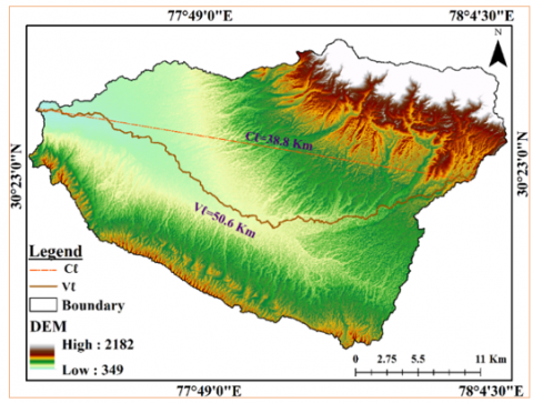
Various researchers have briefly described and formulated Mueller’s sinuosity index, including [17, 55-57] has redefined this parameter to integrate hydraulics sinuosity (which is developed by a channel not influence any alignment related to valley-wall) and topographic sinuosity (which is disseminated by valley geometry). The hydro-geomorphic condition of the river, as well as other factors such as terrain characteristics, cause it to deviate from its previous path, which is well measured by ‘$C_{S I}$’. Figure 10, depicts the location of the valley and the length of the channel in the watershed.
Figure 10. Channel Sinuosity Index showing Channel length ($C_l$) and Valley length ($V_l$)
The value of ‘$C_{S I}$’ calculated for the mainstream of the Asan River using the equation proposed by the study [17] is 1.3. This conventional classification suggests that the stream has a braided course (Table 6). The sinuosity of the river is dependent upon underlying topography which includes rock type and structure, climate and vegetation that dominate the area, the impact of different hydrological factors viz., evapotranspiration, precipitation, rainfall, temperature etc., sediment deposition in the course of the river channel.
5.2.4 Basin Shape Index ($B_s$)
The Basin Shape Index ($B_s$) was proposed by the study [14]. In tectonically active areas, it is one of the most important parameters for determining the relatively younger drainage basin. Basin shape influences the fluxes, runoff and sediment from headwater reaches. In the tectonically active area, the relatively younger watershed is elongated in a shape corresponding to the topographic slope or young active fault [14]. In the present study, the classification proposed by the study [58] is adopted. The calculated value of the ‘$B_s$’ for Asan watershed is 1.4 suggesting that the shape of the watershed is elongated and tectonically active (Table 6). This conversion in the shapes of the watershed is because the width of the watershed is narrower near the mountain front in the actively tectonic area.
5.2.5 Stream Length to Height Ratio ($S L_{index}$)
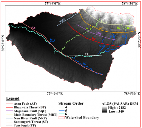
Stream Length to Height Ratio ($S L_{index}$) was given by the study [16]. The variation in channel gradient affects the $S L_{index}$ and this effect helps to evaluate the tectonism in an area. River gradient also reflects the variation of lithology and is an indication of the tectonically disturbed river [55, 59]. The structural features such as fault and structural lines are consistent with the steep slope. It also helps to evaluate relative tectonic activity. Various tectonic, lithological and/or climatic factors are responsible for the deviation of river profile [16]. In the present study, $S L_{index}$ is computed using DEM. For every 200m elevation difference, the distance from the source is determined in a GIS environment [59]. The main tributary stream of the 6th order, five streams of the 5th order and three streams of the 4th order are taken for the calculation of $S L_{index}$ (Figure 11).
Figure 11. Location of the 4th, 5th and 6th ordered stream taken for the analysis of stream length ratio along with major faults and thrust
The longitudinal profile for corresponding streams and numerous pronounced topographic break or knick point distributions along the profile in the middle and upper reaches of all the prominent streams of the study area are shown in Figure 12. These breaks or knick points help in examining the polycyclic nature of landform development and are influenced by major tectonic structures (fault and thrust) present in the area.
Based on the categorization of highest to lowest values of $S L_{index}$ (Table 6). The average value of $S L_{index}$ for the selected streams is 531, which indicates that the watershed is tectonically active. The $S L_{index}$ is high where the channels flow over active uplifts and cross the soft rocks e.g., alluvial. Conversely, lesser $S L_{index}$ indicates low tectonic activity and also rivers flow over less-resistant harder underlying rocks [60] e.g., Doon gravels. The break distribution shown in Figure 12, is theoretically influenced by faulting or upliftment of bedrock due to tectonic activity, base-level variation due to quaternary climatic deviation and contrasting lithology behaviour of soft and hard bedrocks [61].
The first stream of the 4th order designated as ‘4(1)’, reflects the stream-wise value varies from 0.5-397.5 m and the higher peaks of the profile of stream are flowing across the Bhauwala Thrust (BT), Majahaun Fault (MJF), Santaugarh Thrust (ST) and Main Boundary Thrust (MBT). The second stream of the 4th order ‘4(2)’, reflects the stream-wise value varies from 1-347.5m and the higher peaks on the stream’s profile are traverse across the Main Boundary Thrust (MBT). The third stream of the 4th order designated as ‘4(3)’, reflects the stream-wise value varies from 0.5-685m and the higher peaks on the stream’s profile traverse across the Main Boundary Thrust (MBT). The first stream of the 5th order designated as ‘5(1)’, reflects the stream-wise value varies from 1-138m and the higher peaks on the stream’s profile are traverse across Asan Fault (AF). The second stream of the 5th order ‘5(2)’, reflects the stream-wise value varies from 1-322m and the higher peaks on the stream’s profile are traversed across the Asan Fault (AF). The third stream of the 5th order designated as ‘5(3)’, reflects the stream-wise value varies from 1-758m and the higher peaks on the stream’s profile are traversed across Tons Fault (TF) and Bhauwala Thrust (BT). The fourth stream of the 5th order ‘5(4)’, reflects the stream-wise value varies from 1-680m and the higher peaks on the stream’s profile are traversed across the Bhauwala Thrust (BT), Majahaun Fault (MJF), Santaugarh Thrust (ST). The fifth stream of the 5th order ‘5(5)’, reflects the stream-wise value varies from 1-780m and the higher peaks on the stream’s profile are traversed across the Bhauwala Thrust (BT) and Santaugarh Thrust (ST). The stream-wise mean value of $S L_{index}$ varies from 0.5 to 566m for the Asan River (mainstream) of the 6th order of stream network. The higher peaks on the stream’s profile are traversed across the Asan Fault (AF) and Tons Fault (TF). Increasing the level of erosion, this fault and thrust zones along the river’s course may cause landslides.
Figure 12. Longitudinal river profile and $S L_{index}$ of the fourth, fifth and sixth ordered streams (BT-Bhauwala Thrust; ST-Santaugarh Thrust; MF-Majahaun Fault; TF-Tons Fault; AF-Asan Fault; MBT-Main Boundary Thrust)
5.3 Terrain attributes
5.3.1 Slope
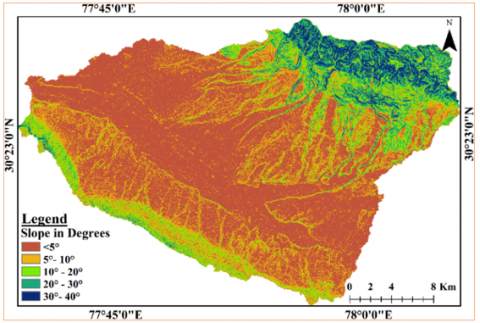
The slope is one of the significant features of the earth’s surface required for hydrological study in the area. Slope measures the steepness of the surface (in degrees or percent rise) at any particular location. Several researchers such as the studies [57, 62-66] proposed various methods for expressing slope. In geomorphology, the slope is an amalgamation of ‘form' and ‘process' which includes geology, climate, vegetal cover and process of weathering respectively. In the present study, slope maps are generated from DEM using the surface analyst module in ArcMap v.10.3 (Figure 13). The entire slope range has been divided into five classes ranging from 5° to 40°. The classification presents a better picture of slope distribution in the area. This classification is adopted from the report of ‘The Commission on Slope Evolution’ published in the study [67]. The steepness of the slope is expressed by its saturation-steeper slopes have brighter colours.
Figure 13. Slope map
Table 9. Slope classes and their aerial extent of the study area
|
S.N |
Slope Class |
Range of Slope |
Utility/ Problem |
Area (sq.km) |
Percent Area |
Cumulative Percent |
|
1 |
Gentle |
<5° |
Agriculture, Forestry, Good for walking, road transport and railway construction. |
361.6 |
51.9 |
51.9 |
|
2 |
Moderate |
5°-10° |
Difficulties for road building. 120-150 limit for settlement and industries. |
148.7 |
21.4 |
73.3 |
|
3 |
Moderate Steep |
10°-20° |
Road transport only for special vehicles. Limited possibility for construction. |
98.1 |
14.1 |
87.4 |
|
4 |
Steep |
20°-30° |
No possibility of agriculture or building. |
50.3 |
7.2 |
94.6 |
|
5 |
Very Steep |
30°-40° |
No cultivation, walking difficult. Mostly forests but also limit of utilization in forestry. |
37.3 |
5.4 |
99.9 |
|
Total |
|
|
|
695.9 |
99.9~100 |
100 |
Table 9 portrays the areal distribution of each slope category, the range of slope and the frequencies of individual slope classes. Around 73.3% of the area in the watershed belongs to a moderate to gentle slope where settlement and industries are predominant (Figure 3(b)). Because of the slightly undulating topography, moderate slopes have a good infiltration zone that leads to maximum infiltration or partial runoff. The northern part of the watershed which mostly comprises rocks of Lesser Himalayan formation such as quartzite, phyllite, limestone, and dolomite of the Chandpur, Nagthat, Blaini, Krol and Tal formation has a steep slope whereas the areas of flat terrain with gentle slope are characterised by river terraces, old landslide debris, saddles, fluvial fan and so on.
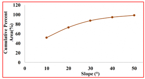
The spatial distribution of slope in degrees concerning the areal coverage and cumulative percentage is shown in Figure 14. The y-axis of a frequency curve corresponds to the cumulative percent area of slope classes while the x-axis corresponds to the cumulative slope in degrees. The area under the curve, as calculated from the graph was 91.2% accurate. In the Siwalik zone, because of the presence of a dominantly steep slope, the fans create piedmont zones along the southern periphery and moderately dipping beds are visible where water quickly runoff.
Figure 14. Cumulative frequency distribution for Slope
The northern part of the watershed mostly comprises rocks of Lesser Himalayan formation such as quartzite, phyllite, limestone, and dolomite of the Chandpur, Nagthat, Blaini, Krol and Tal formations have a steep slope, whereas the relatively flat and gently sloping areas are characterized by deep weathering, bulges of old landslide debris, river terraces and fluvial fan. In the Siwalik zone, because of the presence of a dominantly steep slope, the fans forming the piedmont zone along the southern fringes of the watershed and moderate to a steep dip of the bed are seen where water quickly runoff.
Figure 15. Slope-aspect map
5.3.2 Slope-aspect analysis
The steepest slope direction for a location on the surface is measured by an aspect map. The aspect map is a critical parameter for determining the impact of the sun on the local climate. In most cases, the west-facing slope will be warmer than the east-facing slope during the hottest part of the day. As a result, the aspect has a significant impact on the spread of vegetation types in the area. Aspect is the angle between the vertical directions of the steepest slope, it is always measured in a clockwise direction. Like Slope, the Aspect is also calculated from DEM (ALOS-PALSAR) and usually measured in degrees. As shown in Figure 15, the aspect categories are represented by hues (e.g., red, orange, yellow, etc.) and the degree of slope classes are mapped with saturation (or colour brilliance) so that the steeper slopes are brighter.
The aerial and frequency distribution of the aspect categories is shown in Table 10. The aspect reclassify values are designated the corresponding distribution of aspect classes.
There is a close relationship between aspects, landform types and natural vegetation in the study area. It is noted from Table 10, that the northern aspect of the watershed is steeper than the southern aspect. The north-western aspect is good for biodiversity. The curve represents the relationship between the cumulative area and aspect reclassify value increasing toward the right showing an accuracy of 98% (Figure 16).
The direction of the vegetation and forest growth are good indicators of the aspect. In the higher reaches of the watershed, the density of oak and associated species like Cupressus are well developed in the north-western aspect while the pine is well dominated in the south-eastern one.
Figure 16. Cumulative frequency distribution for Slope-aspect
5.4 Land use/land cover mapping
The most important factors in determining the topographical features and status of classes in the watershed are changes in land use and land cover patterns. Estimation and change in land use patterns suggest resource utilization through human interferences especially utilizing urbanization and agriculture [68]. LULC becomes a significant aspect of the monitoring of different hydrological processes and natural resources management [5, 20, 21].
In the present paper, the LULC mapping for the years: 1980, 1995, 2008 and 2016 is prepared through visual interpretation of geo-referenced satellite images of Landsat and LISS-IV (data description mentioned in Table 4) using ArcMap v.10.3 and ERDAS IMAGINE. The on-screen interpretation is carried out on a scale of 1:10,000. The map thus generated was taken to the field for verification and the final vector polygon map depicting the various land use/land cover classes in the study area was prepared [22]. The digitization of the different classes of LULC is based on the classification given by the studies [69, 70]. It is classified into eight different classes: built-up (urban and rural), cropland, fallow land, plantation, evergreen needle leaf forest, deciduous broadleaf forest, mixed forest, and water bodies (Figure 6).
Remote sensing is also used in hydrologic analysis to investigate the impact of changing land-use patterns (e.g., agricultural pattern, forest coverage, urbanization and so on) on various hydrologic responses of the watershed. Table 11, shows the different classes of LULC used in the study.
In 1980, the urban area of the watershed occupied 9.13Km2 (10.38%) which increased by 2.40% in 1995 to reach 11.71 Km2 as revealed in Figure 17 and Table 12. The continuous urban areal increment is visible in 1995-2008 with a 12.39 Km2 increase in area to reach 24.43 Km2 (30.11%) in 2008 and 11.07 Km2 of areal increment of 35.50 Km2 (45.79%) in 2016.
Figure 17. Percentage of urban growth in the area
5.4.1 Areal distribution of LULC classes
Areal statistics of different classes of LULC are given in Table 1, which corresponds to the dominance of forest class in the watershed followed by agriculture and built-up.
Table 10. Slope-aspect categories and their aerial extent
|
S.N. |
Aspect Classes |
Division of Aspect Classes (°) |
Aspect Reclassify Value |
Area (sq.km) |
Percent Area (%) |
Cumulative Percent |
|
1 |
Flat |
0° |
1 |
99.79 |
14.34 |
14.34 |
|
2 |
North |
0°-22.5° |
2 |
58.71 |
8.44 |
22.78 |
|
3 |
Northeast |
22.5°-67.5° |
3 |
57.63 |
8.28 |
31.06 |
|
4 |
East |
67.5°-112.5° |
4 |
66.84 |
9.60 |
40.66 |
|
5 |
Southeast |
112.5°-157.5° |
5 |
55.30 |
7.95 |
48.61 |
|
6 |
South |
157.5°-202.5° |
6 |
77.51 |
11.14 |
59.75 |
|
7 |
Southwest |
202.5°-247.5° |
7 |
72.20 |
10.38 |
70.12 |
|
8 |
West |
247.5°-292.5° |
8 |
72.79 |
10.46 |
80.58 |
|
9 |
Northwest |
292.5°-337.5° |
9 |
80.67 |
11.59 |
92.18 |
|
10 |
North |
337.5°-360° |
10 |
54.54 |
7.84 |
100.01 |
|
Total 695.9 |
100 |
100 |
||||
The result indicates that there is a significant change in the LULC classes of built-up and plantation. It is found that in the years 1980, 1995, 2005 and 2016 the total built-up area which includes rural and urban settlement covers 9.13 Km2 in 1980 to 35.50 Km2 in 2016. It covers 1.31% to 5.10% of the total area of the watershed. On the contrary, the percentage of plantations in the watershed decreases from 3.23% to 2.13% of the watershed. The area of water bodies that covers the watershed also decreases. This is because of the rapid increase in urbanization, industrialization, and population in the watershed over the past decades with an additional requirement for food and shelter. These surface areas are increasing by decreasing forest surface as well as total forest surface and water bodies. The watershed is also facing a problem of high erosion as a result of intense rainfall and LULC change.
Table 11. Different classes of LULC with description [69, 70]
|
S.No. |
Land Cover |
Description |
|
1. |
Settlement |
|
|
2. |
Agriculture |
|
|
3. |
Fallow land |
|
|
4. |
Rangeland |
|
|
5. |
Forest |
|
|
6. |
Waterbodies |
|
Table 12. Urban growth of the Asan watershed (1980-2016)
|
Year |
Urban Area (Km2) |
Urban Area Change (%) |
Increase (Km2) |
|
Till 1980 |
9.13 |
10.38 |
- |
|
1980-1995 |
11.71 |
13.83 |
2.40 |
|
1995-2008 |
24.43 |
30.11 |
12.39 |
|
2008-2016 |
35.50 |
45.01 |
11.07 |
Further, the results validated from field studies, the dislocation of jointed and weathered rocks due to the presence of slopes in the Lesser Himalayan region resulted in the activation of mass wasting in the area. The deflection and shifting of the water body and the development of flood plains, deposition of sand and landforms on both sides of the river (Figure 18). These examples interpret major pieces of evidence and the parameters which are studied in the research determine the decisive factors for the presence of tectonics in the area. The outburst of population and settlement in the entire region of the watershed particularly in the Lesser Himalayan region confirms their decadal increment. The continuous drying of water bodies over time and changes in LULC's classes have impacted the water balance of the watershed by changing the magnitude of flow, which results in increasing the extent of the water management problem.
Figure 18. Different activities responsible to make watershed fragile and controlled
Geomorphic indices related to drainage network analysis provide a quantitative description of the stream network which gives significant information about the characterization of the watershed. Evaluation of these indices is critical for maintaining the sustainable development of water resources in the area. Both the surficial and sub-surficial characteristics of the watershed are revealed through these indices. The watershed dynamics are studied by 24 indices which include 19 morphometric and 5 morphotectonic ones. The study reveals that the stream network exhibits dendritic and trellis patterns, and extends to 6th order. Lower-order streams mostly dominate the watershed covering the largest draining area. The bifurcation ratio for the 6th ordered stream network indicates its value ranges from 3-5 for the entire watershed. The higher value of the bifurcation ratio ($R_b$) infers to the comparatively younger stage of stream development and the influence of structural features in the area. The Asan River (6th order mainstream) passes through the Asan Fault (AF) represents the higher value of ‘$R_b$’. On the contrary, the mean bifurcation ratio ($R_{bm}$) suggests that the overall influence of geological structure on the drainage pattern of the watershed is minimal. The watershed is drained by the moderately permeable strata with medium run-off and infiltration capacity, as evidenced by the moderate range of drainage density $\left(D_d\right)$ and drainage texture $\left(D_t\right)$. The area has moderate stream frequency $\left(F_s\right)$ which reflects the moderate ground slopes, rock permeability, run-off and infiltration capacity of the watershed. Elongation ratio $\left(R_e\right)$ suggests that the shape of the watershed is elongated. The length of the flow path $\left(L_q\right)$ shows a well-developed stream network with moderate slopes showing surface runoff travels at a relatively shorter distance before flowing through the channels.
From the relief aspect, it is found that the maximum height of the watershed covers the Lesser Himalaya ranges with the minimum area and the least elevation is seen in a nearby position of the mouth of the watershed. The relief ratio ($R_h$) suggests that the presence of moderate to gentle slopes and less resistant rocks in the area increases the discharge capacity and lowers the groundwater potential of the area. Additionally, the basement rocks exposed as small ridges and mounds have a lower slope effect, allowing moderate runoff and erosion. The calculated value of the Ruggedness number ($R_n$) suggests that the watershed has a rugged topography with moderately high conditions of soil erosion and flood potential.
Asymmetry factor ($A_f$) gives significant information about the presence of tectonic tilt in the area and shows structural discontinuity as it passes through major thrust/faults. The observed absolute value of ‘$A_f$’ categorized the watershed into gently asymmetrical. The evaluation of Hypsometric integral ($H_i$) reveals that the convex-concave/S-shaped hypsometric curve is associated with a mature stage of stream development corresponding to the presence of moderately eroded strata and dissected drainage network in the area. The Coefficient of determination (R2) obtained from the Hypsometric curve of the watershed reveals that the watershed is sufficiently adjusted towards the prevailing conditions. The mainstream follows the braided course and is reflected through the Channel Sinuosity Index ($C_{S I}$). The shape and degree of activeness of the region are observed by the Basin Shape Index ($B_s$). Based on the classification, the Asan watershed exhibits an elongated shape. The more elongated the shape of the watershed, the more active the region. Stream length to height ratio ($S L_{\text {index }}$) is calculated for the major stream of the 6th order, five streams of the 5th order and three streams of the 4th order at an interval of 200m elevation difference from the source and it reveals the influence of geological structures such as several faults and thrust affecting the shape of the longitudinal profile, at the drainage region of the watershed. The intersection of the longitudinal profile along the streams may indicate some upliftment in the topography due to significant tectonic disturbances. Lithological discontinuities and tectonic uplift have resulted in the development of knick-points and anomalously high values of $S L_{\text {index }}$.
The slope and aspect in the area create a huge impact on the stream network development. From the slope analysis, it is indicated that the maximum area of around 73.3% of the total watershed area belongs to a moderate to gentle slope (<5°-10°) with the predominance of settlement and industries. The dominance of moderate to gentle slopes in the watershed gives good support to the infiltration rate. The aspect shows overestimation in total areal coverage around 99.79Km2 ~ 14.34% flat followed by 80.67Km2 ~ 11.59% northwest aspect. The north-western aspect is good for biodiversity. The aspect map suggests that the northern aspect of the watershed is steeper than the southern aspect. In the high altitude, the growth and density of oak and associated species like Cupressus are well in the northern and western aspects while the pine is well dominated in the south-eastern aspects.
Hydrological dynamics in a river watershed are altered by LULC change. The LULC shows the changing scenario (through decades) of the watershed. It shows the dominance of forest cover followed by agricultural and built-up areas, particularly in the northern and southern parts of the watershed. The built-up class from LULC maps of 1980, 1995, 2008 and 2016 revealed that the area increased by four times in as many decades (from 1980 to 2016). It is because the watershed along the entire Doon Valley has changed its status and the government has attracted a large number of institutional and commercial activities to come up in the area. The unprecedented growth of the urban area has resulted in chaos, traffic congestion, overcrowding and mass encroachments on the drainage system of the watershed.
The entire study is based on various geo-environmental factors that have long-term effects on the watershed. The hydrological behaviour, evolutionary background, and maturity of the terrain are revealed by the quantitative geomorphometric analysis of the study area. These are all crucial in classifying landforms into different morpho-units and determining how they relate to local geology. The overall investigation demonstrates that the watershed's drainage system is transitioning from an early to a mature stage of the fluvial geomorphic cycle. The area is tectonically active, according to the analysis of geomorphic indices. The experts are very concerned about the 36-year spatial variation in the LULC classes, particularly the four-fold expansion of the built-up area, and this study directly supports a strong need in this regard. This study directly supports the need for sustainable watershed development and management because of the 36-year spatial variation in the LULC classes, especially the four-fold expansion of the built-up area.
The overall study recommends that, to maintain sustainable development, the rate of urban growth in the watershed should be slowed and the spatial pattern of growth should be changed. Altogether, this study mainly relates to soil and water conservation in the watershed, which includes appropriate land use, runoff prevention, improvement of forests and grasslands, protection of water supply, management of local water for irrigation, and enhancement of soil fertility.
By integrating the findings from geomorphic studies, morphometric parameters, and LULC analysis, our paper provides valuable insights into the intricate relationship between human activities and natural processes in the watershed. These insights can be used to develop effective management and conservation strategies, ensuring the sustainable development of the entire area. Also, the study offers useful guidance to watershed managers in making decisions during the planning phase as well as in monitoring and assessing watershed management initiatives.
I declare that this research article is the original part of my research, has been written by me and it is neither published elsewhere nor under review. The experimental work is almost entirely my work; the collaborative contributions have been indicated clearly and acknowledged.
I would like to thank my mentor Dr. Dhirendra Singh Bagri for his guidance in writing the research. His guidance, advice and constructive criticism are highly appreciated. Also, I exceedingly benefitted from his critical thinking, uncertainty assessment and technical writing ability. This work uses datasets from the United States Geological Survey, USGS (https://earthexplorer.usgs.gov/); National Remote Sensing Centre, Bhuvan-NRSC (https://bhuvan.nrsc.gov.in/home/index.php); Earth Observation Research Centre-Japan Aerospace Exploration Agency and Alaska Satellite Facility, ASF (https://asf.alaska.edu/data-sets/derived-data-sets/alos-palsar-rtc/alos-palsar-radiometric-terrain-correction/), are duly acknowledged.
The authors received no specific funding or research grant for this work from any agency in the public, commercial, or not-for-profit sectors, that could have influenced its outcome.
Conceptualization and design of the article; acquisition, methodology, interpretation and validation of the data, formal analysis, writing and original draft preparation-A.S.; Visualization, writing-review and editing-D.S.B.
I testify on behalf of my co-author that our research article is original and is neither published elsewhere nor under review. There is no conflict of interest associated with this research work.
The author used datasets from the United States Geological Survey, USGS (https://earthexplorer.usgs.gov/); National Remote Sensing Centre, Bhuvan-NRSC (https://bhuvan.nrsc.gov.in/home/index.php); Earth Observation Research Centre-Japan Aerospace Exploration Agency, EORC-JAXA (https://www.eorc.jaxa.jp/ALOS/en/aw3d30/index.htm) and Alaska Satellite Facility, ASF (https://asf.alaska.edu/data-sets/derived-data-sets/alos-palsar-rtc/alos-palsar-radiometric-terrain-correction/) to conduct the current research.
[1] Singh, A.K. (1998). Geomorphology, sedimentology and pedology of the intermontane Dehradun Valley, Northwest Himalaya. Unpublished Ph.D. thesis, University of Roorkee, p. 247. http://localhost:8081/xmlui/handle/123456789/897.
[2] Strahler, A. (1964). Quantitative geomorphology of drainage basin and channel networks. In: Chow, V. (Ed.). New York: Handbook of Applied Hydrology, McGraw Hill, New York, 439-476. https://cir.nii.ac.jp/crid/1572824500442828288.
[3] Smith, G.H. (1938). The morphometry of landscape: An analysis of slope. Annals of Association of American Geographers, 29: 34.
[4] Horton, R.E. (1945). Erosional development of streams and their drainage basins; Hydrophysical approach to quantitative morphology. Geological Society of America Bulletin, 56(3): 275-370. https://doi.org/10.1130/0016-7606
[5] Rawat, J.S., Biswas, V., Kumar, M. (2013). Changes in land use/cover using geospatial techniques: A case study of Ramnagar town area, district Nainital, Uttarakhand, India. The Egyptian Journal of Remote Sensing and Space Science, 16(1): 111-117. https://doi.org/10.1016/j.ejrs.2013.04.002
[6] Strahler, A.N. (1952). Dynamic basis of geomorphology. Geological Society of America Bulletin, 63: 923-938. https://doi.org/10.1130/00167606(1952)63[923:DBOG]2.0.CO;2
[7] Strahler, A.N. (1968). Quantitative geomorphology. In: Fairbridge, R.W., Ed., The Encyclopedia of Geomorphology, Reinhold Book Crop., New York.
[8] Grohmann, C.H., Riccomini, C., Alves, F.M. (2007). SRTM-based morphotectonic analysis of the Pocos de Caldas Alkaline Massif, southeastern Brazil. Computers & Geosciences, 33: 10-19. https://doi.org/10.1016/j.cageo.2006.05.002
[9] Pankaj, A., Kumar, P. (2009). GIS-based morphometric analysis of five major sub-watersheds of Song River, Dehradun District, Uttarakhand with special reference to landslide incidences. Journal of the Indian Society of Remote Sensing, 37(1): 157-166. https://doi.org/10.1007/s12524-009-0007-9
[10] Singh, P., Gupta, A., Singh, M. (2014). Hydrological inferences from watershed analysis for water resource management using remote sensing and GIS techniques. The Egyptian Journal of Remote Sensing and Space Science, 17: 111-121. https://doi.org/10.1016/j.ejrs.2014.09.003
[11] Jahan, C.S., Rahaman, M.F., Arefin, R., Ali, S., Mazumder, Q.H. (2018). Morphometric analysis and hydrological inference for water resource management in Atrai-Sib River basin, NW Bangladesh using remote sensing and GIS technique. Journal of the Geological Society of India, 91(5): 613-620. https://doi.org/10.1007/s12594-018-0912-z
[12] Singh, P., Gupta, A., Singh, M. (2014). Hydrological inferences from watershed analysis for water resource management using remote sensing and GIS techniques. The Egyptian Journal of Remote Sensing and Space Science, 17: 111-121. https://doi.org/10.1016/j.ejrs.2014.09.003
[13] Bull, W.B. (2007). Tectonic Geomorphology of Mountains: A New Approach to Palaeo-Seismology. Blackwell Publishing http://doi.org/10.1002/9780470692318
[14] Bull, W.B., McFadden, L.D. (1977). Tectonic geomorphology north and south of the Garlock Fault, California. In: Doehring DO (ed) Geomorphology in arid regions. Publications in Geomorphology. Proceedings volume of the 8th Annual Geomorphology Symposium, State University New York, Binghamton, pp. 118-138. https://doi.org/10.4324/9780429299230
[15] Cox, R.T. (1994). Analysis of drainage-basin symmetry as a rapid technique to identify areas of possible Quaternary tilt-block tectonics: An example from the Mississippi Embayment. Geological Society of America Bulletin, 106: 571-581. https://doi.org/10.1130/0016-7606(1994)106<0571:AODBSA>2.3.CO;2
[16] Hack, J.T. (1973). Stream-profile analysis and stream-gradient index. Journal of Research of US Geological Survey, 1: 421-429.
[17] Mueller, J.E. (1968). An introduction to the hydraulic and topographic sinuosity indexes. Annals of the Association of American Geographers, 58: 371-385. https://doi.org/10.1111/j.1467-8306.1968.tb00650.x
[18] Miller, V.C. (1953). A quantitative geomorphic study of drainage basin characteristics in the clinch mountain area Virginia and Tennessee. Technical report, Columbia University, New York. https://doi.org/10.1086/626413
[19] Nag, S.K. (1998). Morphometric analysis using remote sensing techniques in the Chaka sub-basin, Purulia district, West Bengal. Journal of the Indian Society of Remote Sensing, 26: 69-76. https://doi.org/10.1007/BF03007341
[20] Abebe, G., Getachew, D., Ewunetu, A. (2022). Analysing land use/land cover changes and its dynamics using remote sensing and GIS in Gubalafito district, Northeastern Ethiopia. SN Applied Sciences, 4: 30. https://doi.org/10.1007/s42452-021-04915-8
[21] Sylla, L., Xiong, D., Zhang, H.Y., Bangoura, S.T. (2012). A GIS technology and method to assess environmental problems from land use/cover changes: Conakry, Coyah and Dubreka region case study. The Egyptian Journal of Remote Sensing and Space Science, 15(1): 31-38. https://doi.org/10.1016/j.ejrs.2011.12.002
[22] Sharma, A., Bagri, D.S. (2020). Monitoring of urban sprawl and spatio-temporal variability of landuse/landcover change in Asan watershed, Doon valley, Uttarakhand, India. In AGU Fall Meeting 2020. https://doi.org/10.1002/essoar.10505204.1
[23] Chauhan, M. (2010). A perspective on watershed development in the Central Himalayan state of Uttarakhand, India. International Journal of Ecology and Environmental Sciences, 36(4): 253-269.
[24] Sharma, A., Nikam, B.R., Bagri, D.S., Kumar, D. (2020). Trend analysis of annual and seasonal time series over the last 46 years in Asan Watershed, Doon Valley based on gridded data set. Earth ScienceIndia, 13(1). https://doi.org/10.31870/ESI.13.1.2020.2
[25] Sharma, A., Nikam, B.R., Bagri, D.S., Kumar, D. (2021). Geo-environmental investigations in the Asan River watershed of Doon Valley, Uttarakhand; PhD thesis submitted to HNB GarhwalUniversity/IIRS-ISRO, Dehradun; https://shodhganga.inflibnet.ac.in:8443/jspui/handle/10603/401114.
[26] Kedareswarudu, U., Kumar, S. (2013). Estimation of contribution of springs to Asan River watershed of Doon valley through baseflow-Hydrograph Method. International Journal of Geology, Earth and Environmental Sciences, 3: 69-82.
[27] Jain, C.K., Bhatia, K.K., Sharma, M.K. (1997). Ground Water Quality Evaluation in Doon Valley (p. 37). Dehradun. Report no. CS (AR) 10/96–97, National Institute of Hydrology, Roorkee. http://117.252.14.242/Gangakosh/Publications/NIH_Publications/CS(AR)-10-96-97.pdf.
[28] SSAP. (2018). State Specific Action Plan (SSAP) for Water Sector in Uttarakhand. Report draft of Ministry of Environment, Forest and Climate Change, National Water Mission. https://nwm.gov.in/sites/default/files/Report_Draft-SSAP_Uttarakhand.pdf.
[29] Joshi, B. (2018). Recent trends of rural out-migration and its socio-economics and environmental impacts in Uttarakhand Himalaya. Journal of Urban and Regional Studies on Contemporary India, 4(2): 1-14.
[30] Jasrotia, A.S., Kumar, A., Aasim, M. (2011). Morphometric analysis and hydrogeomorphology for delineating groundwater potential zones of Western Doon Valley, Uttarakhand, India. International Journal of Geomatics and Geosciences, 2: 1078-1096.
[31] Jasrotia, A.S., Bhagat, B.D., Kumar, A., Kumar, R. (2013). Remote sensing and GIS approach for delineation of groundwater potential and groundwater quality zones of Western Doon Valley, Uttarakhand, India. Journal of the Indian Society of Remote Sensing, 41: 365-377. https://doi.org/10.1007/s12524-012-0220-9.
[32] Singh, A.K., Parkash, B., Mohindra, R., Thomas, J.V., Singhvi, A.K. (2001). Quaternary alluvial fan sedimentation in the Dehradun valley piggyback basin, NW Himalaya: tectonic and palaeoclimatic implications. Basin Research, 13: 449-471. https://doi.org/10.1046/j.0950-091x.2001.00160.x
[33] Raiverman, V., Kunte, S.V., Mukherjea, A. (1984). Basin geometry, Cenozoic sedimentation and hydrocarbon prospects in northwestern Himalaya and Indo-Gangetic plains. Petroleum Asia Journal, 6: 67-92.
[34] Sinha, S., Sinha, R. (2016). Geomorphic evolution of Dehra Dun, NW Himalaya: Tectonics and climatic coupling. Geomorphology, 266: 20-32. https://doi.org/10.1016/j.geomorph.2016.05.002
[35] Valdiya, K.S. (1980). The two intracrustal boundary thrusts of the Himalayas; Tectonophysics, 66: 323-348. https://doi.org/10.1016/0040-1951(80)90248-6
[36] Thakur, V.C., Pandey, A.K. (2004). Active deformation of Himalayan Frontal Thrust and Piedmont zone south of Dehradun in respect of seismotectonics of Garhwal Himalaya. Himalayan Geology, 25: 23-31.
[37] Thakur, V.C. (1995). Geology of Dun Valley, Garhwal Himalaya: Neotectonics and coeval deposition with fault-propagation folds. Himalayan Geology, 6(2): 1-8.
[38] Ahmad, S., Bhat, M.I., Madden, C., Bali, B.S. (2014). Geomorphic analysis reveals active tectonic deformation on the eastern flank of the Pir Panjal Range, Kashmir Valley, India. Arabian Journal of Geosciences, 7(6): 2225-2235. https://doi.org/10.1007/s12517-013-0900-y
[39] Lambert, D. (1998). The Field Guide to Geology. 130-131. Checkmark Books.
[40] Schumm, S.A. (1956). Evolution of drainage systems and slopes in badlands at Perth Amboy, New Jersey. Geological Society of America Bulletin, 67(5): 597-646. https://doi.org/10.1130/0016-7606(1956)67[597:EODSAS]2.0.CO;2
[41] Shukla, D.P., Dubey, C.S., Ningreichon, A.S., Singh, R.P., Mishra, B.K., Singh, S.K. (2014). GIS-based morpho-tectonic studies of Alaknanda river basin: A precursor for hazard zonation. Natural Hazards, 71: 1433-1452. https://doi.org/10.1007/s11069-013-0953-y
[42] Iron, Z. (1985). Basin Hydrology. Retrieved from https://www.sciencedirect.com/science/article/pii/S0167564808704131on 23/03/2019.
[43] Horton, R.E. (1932). Drainage basin characteristics. Transactions of the American Geophysical Union, 13: 350-361. (https://doi.org/10.1029/TR013i001p00350
[44] Vittala, S.S., Govindaiah, S., Gowda, H.H. (2004). Morphometric analysis of sub-watersheds in the Pavagada area of Tumkur district, South India using remote sensing and GIS techniques. Journal of the Indian Society of Remote Sensing, 32: 351-362. https://doi.org/10.1007/BF03030860
[45] Cannon, P.J. (1976). Generation of explicit parameters for a quantitative geomorphic study of the Mill Creek drainage basin. Oklahoma Geology Notes, 36(1): 3-16.
[46] Mayomi, I.Y. (2018). Geospatial analysis of morphometric characteristics of river Hawul basin, north-east Nigeria. Resources and Environment, 8(3): 103-126.
[47] Hare, P.W., Gardner, T.W. (1985). Geomorphic indicators of vertical neotectonism along converging plate margins, Nicoya Peninsula, Costa Rica. Tectonic Geomorphology, 4: 75-104.
[48] Keller, E., Pinter, N. (2002). Active Tectonics: Earthquakes, Uplift and Landscape. New Jersey.: Prentice-Hall Earth Science Series.
[49] Cuong, N.Q., Zuchiewicz, W.A. (2001). Morphotectonic properties of the Lo river fault near Tam Dao in North Vietnam. Natural Hazards and Earth System Sciences, 1: 15-22. https://doi.org/10.5194/nhess-1-15-2001
[50] Molin, P., Pazzaglia, F.J., Dramis, F. (2004). Geomorphic expression of active tectonics in a rapidly-deforming forearc, Sila massif, Calabria, southern Italy. American Journal of Science, 304(7): 559-589. https://doi.org/10.2475/ajs.304.7.559
[51] Perez-Pena, J.V., Azor, A., Azanon, J.M., Keller, E.A. (2010). Active tectonics in the Sierra Nevada (Betic Cordillera, SE Spain): Insights from geomorphic indexes and drainage pattern analysis. Geomorphology, 119: 74-87. https://doi.org/10.1016/j.geomorph.2010.02.020
[52] Willgoose, G., Hancock, G. (1998). Revisiting the hypsometric curve as an indicator of form and process in the transport-limited catchment. Earth Surface Processes and Landforms: The Journal of the British Geomorphological Group, 23: 611-623. https://doi.org/10.1002/(SICI)1096-9837(199807)23:7<611::AID-ESP872>3.0.CO;2-Y
[53] Dehbozorgi, M., Pourkermani, M., Arian, M., Matkan, A.A., Motamedi, H., Hosseiniasl, A. (2010). Quantitative analysis of the relative tectonic activity in the Sarvestan area, central Zagros, Iran. Geomorphology, 121: 329-341. https://doi.org/10.1016/j.geomorph.2010.05.002
[54] Bhatta, S.B., Biyani, A.K., Dudeja, D. (2007). Morphometric analysis of lesser himalayan burkot-purola-sandra area of the part of yamuna and tons river basins of uttarkashi district of uttaranchal. Quarterly Journal of Geological Association and Research Centre, Balaghat (M.P.), 15(1): 1-15.
[55] Leopold, L.B., Wolman, M.G. (1957). River channel patterns: braided, meandering, and straight. US Government Printing Office, 282(B): 72-73. https://doi.org/10.3133/pp282B
[56] Haggett, P., Chorley, R.J. (1969). Network Analysis in Geography. London: Edward Arnold. https://escholarship.org/uc/item/7rb9445s.
[57] Pitty, A.F. (1969). A Scheme for Hillslope Analysis. University of Hull publications. No.9, 76. (CRID: 1130000794222399488).
[58] Mahmood, S.A., Gloaguen, R. (2012). Appraisal of active tectonics in the Hindu Kush: Insights from DEM derived geomorphic indices and drainage analysis. Geoscience Frontiers, 3: 407-428. https://doi.org/10.1016/j.gsf.2011.12.002
[59] Sharma, A., Bagri, D.S. (2021). Analysis of tectonic deformation on channel morphology through quantitative geomorphic indices and DEM derived drainage system. Proceedings of the National Academy of Sciences, 87: 283-301. https://doi.org/10.1007/s43538-021-00041-6
[60] Anand, A.K., Pradhan, S.P. (2019). Assessment of active tectonics from geomorphic indices and morphometric parameters in part of Ganga basin. Journal of Mountain Science, 16: 1943-1961. https://doi.org/10.1007/s11629-018-5172-2
[61] Font, M., Amorese, D., Lagarde, J.L. (2010). DEM and GIS analysis of the stream gradient index to evaluate effects of tectonics: The Normandy intraplate area (NW France). Geomorphology, 119(3-4): 172-180. https://doi.org/10.1016/j.geomorph.2010.03.017
[62] Calef, W., Newcomb, R. (1953). An average slope map of Illinois. Annals of the Association of American Geographers, 43: 305-316. https://doi.org/10.1080/00045605309352157
[63] Miller, O.M., Summerson, C.H. (1960). Slope Zone maps. Geographical Review, 50: 194-202. https://doi.org/10.2307/211507
[64] Prasad, N. (1982). Some aspects of meandering streams of the Barakar basin and their sinuosity indexes. In Perspectives in Geomorphology, 4: 93-102. Essay on Indian geomorphology (ed. H.S. Sharma), Concept Publishing Company, New Delhi.
[65] Wentworth, C.K. (1930). A simplified method of determining the average slope of land surfaces. American Journal of Science, 5: 184-194. https://doi.org/10.2475/ajs.s5-20.117.184
[66] Smith, G.H. (1939). The morphometry of Ohio: The average slope of the land. Annals of the Association of American Geographers, 29: 94.
[67] IGU. (1970). Report of the Commission on the slope evolution. Calcutta: National Committee for Geography, Calcutta: International Geographical Congress (IGC).
[68] Singh, P., Thakur, J.K., Kumar, S., Singh, U.C. (2011). Assessment of land use/land cover using geospatial techniques in a semi-arid region of Madhya Pradesh, India. In Geospatial Techniques for Managing Environmental Resources, pp. 152-163. Springer, Dordrecht. https://doi.org/10.1007/978-94-007-1858-6_10
[69] Carnahan, J.A. (1973). International classification and mapping of vegetation, ecology and conservation. Paris: Publication No.6, UNESCO, Paris. Paperback. Cartography, 9(3): 195. https://doi.org/10.1080/00690805.1976.10437920
[70] Ford-Robertson, F.C. (1971). Terminology of forest science, technology practice and products. Society of American Foresters (CRID: 1130000794369336192).