Suman Machavarapu* | Mannam Venu Gopala Rao | Pulipaka Venkata Ramana Rao
OPEN ACCESS
Voltage stability is the most vital phenomena in power systems which may be mainly disturbed by a mismatch in the reactive power generation and load. Not only reactive power imbalance sometimes due to internal faults of the equipments and short circuit faults there may be voltage collapse at the buses. Voltage stability can be enhanced using shunt devices such as Static VAR Compensator (SVC). It can generate or absorb reactive power in a controlled manner such that it can able to enhance Voltage Stability. Voltage Stability Index method is used to determine Voltage sensitivity at each bus and the bus having highest Voltage stability index value can be considered as weak bus which is the optimal location of facts controller. In this paper investigation is made to observe how susceptance model and firing angle model of SVC is used to enhance the voltage at each bus under chaotic load case is observed. IEEE 5-bus and 30-bus systems are considered as test systems and simulations are carried out in Matlab environment.
voltage stability, voltage collapse, voltage sensitivity, voltage stability index, static VAR compensator
Voltage instability is one of the major problems in a modern power system that has been challenging issue for power system engineers for so many decades. Voltage instability leads to Voltage collapse which may in turn leads collapse of the power system. Voltage collapse is highly undesirable in power systems, it occurs when the system is overloaded. The primary reason for Variation in voltage is an imbalance between reactive power generation and consumption.
FACTS devices facilitate an effective solution to prevent Voltage instability and voltage collapse due to their fast and flexible control. FACTS controllers are power electronic devices which are mainly used to improve the power handling capability of the lines by controlling the reactive power.
SVC is the combination of Thyristor Control Reactor (TCR) and Thyristor Switched Capacitor (TSC). SVC can effectively generate or absorb reactive power in a controlled manner.
In different problems of Voltage Stability [1] and how to counteract was described. [2] Deals with the different FACTS controllers and the improvement of the loadability limits of transmission lines. The voltage stability index and how to determine [3] weak bus using voltage stability index. [4] Discussed about the power flow analysis and Newton Raphson power flow algorithm. [5] Presents different models of SVC and incorporating in power system. Describes the voltage stability index [6-7] and Simplified Voltage stability index. Different voltage sensitivity indices are discussed in [8]. [9-10] Deals the susceptance model and firing angle model of SVC FACTS controller and how these models are incorporated in power system. It was clearly given about optimal siting [11] of FACTS controller and also gives how different FACTS controllers improve the voltage profile using reactive power control.
If a right location is selected a single SVC can control voltage stability of all buses. In this paper index method is used to find out the critical or weak buses. If The load at the critical bus is increased beyond the rated level, then there will voltage drop at all the buses which should be compensated SVC FACTS controller. The Effectiveness of SVC Facts controller is observed using susceptance and firing angle models with increased load condition.
Section-2 describes a load flow solution using the Newton Raphson method. The critical or weak bus is identified using Voltage Stability Index approach in section-3. Section-4 presents mathematical modeling of SVC.
Load flow [12] equations are used to determine the best of operation of existing power system and also an extension of the existing power system in a more economical way. Continuous monitoring of power system can be possible by knowing the status of the system time to time. The unknown parameters at the buses there by power flows in the lines and losses can be determined. Newton Raphson (NR) load flow is just like solving a set of nonlinear equations using Newton Raphson method. The NR load flow method is having quadratic convergence characteristics so that it is superior to other load flow methods. This method is more efficient method for large and complex power systems. It needs less number of iterations to reach convergence and the number of iterations is independent of the size of the system.
SVC [13] is the combination of both Thyristor Controlled Reactor (TCR) and Thyristor Switched Capacitor (TSC). TCR can able to provide controlled reactive power absorption and TSC can able to provide controlled reactive power generation. SVC can absorb or generate reactive power in a controlled manner. SVC can be modelled in two ways as given in 4.1 and 4.2
3.1 Susceptance model
In practice the SVC can be seen as an adjustable reactance with either firing angle limits or reactance limits. The equivalent circuit shown in the above figure is used to derive the SVC nonlinear power equations and the linearized equations required by Newton’s method from the above figure the current drawn by the SVC is given by, which is also the reactive power injected at bus k.
$I_{S V C}=j^{*} B_{S V C} * V_{k}$ (1)
and the reactive power drawn by the SVC, which is also the reactive power injected at bus k.
$Q_{S V C}=Q_{k}=-V_{k}^{2} * B_{S V C}$ (2)
The linearised equation is given by the following equation
$\left[\begin{array}{c}\Delta P_{k} \\ \Delta Q_{k}\end{array}\right]^{(i)}=\left[\begin{array}{cc}0 & 0 \\ 0 & Q_{k}\end{array}\right]^{(i)}\left[\begin{array}{c}\Delta \theta_{k} \\ \Delta B_{S V C} / B_{S V C}\end{array}\right]^{(i)}$ (3)
The changing susceptance represents the total SVC susceptance necessary to maintain the nodal voltage magnitude at the specified value.
3.2 Firing angle model
An alternate SVC model, which circumvents the additional iterative process, consists in handling the thyristor – controlled (TCR) firing angle α. In firing angle method BSVC is given by
$I_{S V C}=j * B_{S V C} * V_{k}$ (4)
$\mathrm{B}_{\mathrm{svc}}=\mathrm{B}_{\mathrm{c}}-\mathrm{B}_{\mathrm{TCR}}=-\frac{1}{X_{C} * X_{L}}\left\{X_{L}-\frac{X_{C}}{\Pi} *\left[2 *\left(\prod-\alpha\right)+\sin 2 \alpha\right]\right\}$
$X_{L}=\omega^{*} L$
$X_{C}=\frac{1}{\omega^{*} C}$ (5)
$Q_{k}=-\frac{V_{k}^{2}}{X_{C} * X_{L}}\left\{X_{L}-\frac{X_{C}}{\Pi} *[2 *(\Pi-\alpha)+\sin 2 \alpha]\right\}$ (6)
From equation (9), the linearised SVC equation can be written as
$\left[\begin{array}{c}\Delta P_{k} \\ \Delta Q_{k}\end{array}\right]=\left[\begin{array}{cccc}0 & & 0 & \\ 0 & & \frac{2 * V^{2}}{\Pi * X_{L}} & {[\cos (2 \alpha)-1]}\end{array}\right]\left[\begin{array}{c}\Delta \theta_{k} \\ \Delta \alpha\end{array}\right]$ (7)
L-Index is used to determine weak or critical bus. The bus having highest L-Index[14-15] value can be considered as weak bus. Weak or critical bus is nothing but when ever disturbsnce occurs which bus effects severely.
At load bus VSI can be determind as follows
${{L}_{j}}=\left| {{L}_{j}} \right|=\left| 1-\frac{\sum\limits_{i=1}^{{{\alpha }_{G}}}{{{C}_{ij}}{{V}_{i}}}}{{{V}_{j}}} \right|$ (8)
$\alpha_{G}$ Number of Generator Buses
Vj= Complex voltage at Load j
Vi=Complex voltage at generator bus i
Cij=Elements of matrix C which can be determined using the following equation
$\left[ C \right]=-{{\left[ {{Y}_{LL}} \right]}^{-1}}\left[ {{Y}_{LG}} \right]$ (9)
Sub matrices of YBUS matrix are [YLL ] and [YLG] and it can be found using
$\left[ \begin{matrix} {{I}_{L}} \\ {{I}_{G}} \\\end{matrix} \right]=\left[ \begin{matrix} {{Y}_{LL}} & {{Y}_{LG}} \\ {{Y}_{GL}} & {{Y}_{GG}} \\\end{matrix} \right]\left| \begin{matrix} {{V}_{L}} \\ {{V}_{G}} \\\end{matrix} \right|$ (10)
Two different test systems are considered as given in 5.1 and 5.2
5.1 Test case1: Standard IEEE 5-bus system
Standard IEEE 5-bus sytem is as shown in Figure 1 with one slack bus, voltage control bus and three load buses.
Figure 1. Standard IEEE 5-bus system
The load of the 5-bus is increased up 10% to 200%, and voltage variations at all buses tabulated in Table1.
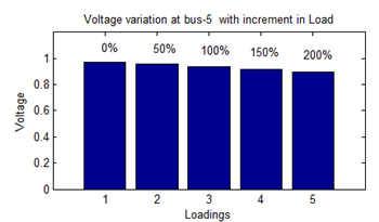
From the Table1 it was clear that with increment in loading the bus voltages keep on decreasing. As the loading of 5th bus increased the voltage at this bus is more effected than other buses which is as given in Figure 2.
Table 1. Variation of bus voltages with respect to increment of load at bus-5
|
Bus .No |
%Change in load Demand |
|||
|
0% |
10% |
50% |
200% |
|
|
1 |
1.05 |
1.05 |
1.05 |
1.05 |
|
2 |
1 |
1 |
1 |
1 |
|
3 |
0.9846 |
0.9839 |
0.9808 |
0.9664 |
|
4 |
0.982 |
0.9811 |
0.9774 |
0.9599 |
|
5 |
0.971 |
0.9679 |
0.9549 |
0.8969 |
Figure 2. Variation in bus-5 voltages with increment in Loading
L-index is calculated at all buses and tabulated in Table 2
Table 2. L-Index values with normal and heavy loading
|
S.No |
Base Loading |
|
|
Bus No. |
(L)Index |
|
|
1 |
5 |
0.1033 |
|
2 |
3 |
0.0601 |
|
3 |
4 |
0.0174 |
From the Table-2 we can observe that at 5th bus L-Index value is 0.1033 which is the highest of all. So the conclusion is 5th bus is weak bus. By varying SVC susceptance, Variations of bus voltages at all buses tabulated in Table 3
Table 3. Improvement in Bus voltages with SVC susceptance
|
Bus .No |
Heavily Loaded case (200%) |
Variation of Bus Voltages with Bsvc |
|||
|
0.3 |
0.6 |
0.9 |
1.106 |
||
|
3 |
0.9664 |
0.9713 |
0.9765 |
0.9818 |
0.9856 |
|
4 |
0.9599 |
0.9662 |
0.9728 |
0.9798 |
0.9847 |
|
5 |
0.8969 |
0.9231 |
0.9505 |
0.9794 |
1 |
From the Table 3 it was observed clearly that By varying susceptance the voltage not only at 5th bus but also at other buses also improved. At susceptance is equal to 1.0106 it was observed exactly the bus-5 voltage is 1 p.u.
By varying the SVC firing angle, Variations of bus voltages at all buses tabulated.
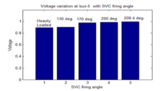
From the Table 4 it was observed that by increasing firing angle not only 5th bus but also voltages of all buses increased. The bus-5 voltage reached to 1 p.u exactly at firing angle 208.40.
Figure 3. Variation in bus-5 voltages with SVC susceptance
Table 4. Improvement in Bus voltages with SVC firing angle
|
Bus .No |
Heavily Loaded case (200%) |
Variation of Bus Voltages with aSVC |
|||
|
130° |
170° |
200° |
208.4° |
||
|
3 |
0.9664 |
0.9679 |
0.9823 |
0.9836 |
0.9856 |
|
4 |
0.9599 |
0.9619 |
0.9804 |
0.982 |
0.9847 |
|
5 |
0.8969 |
0.905 |
0.982 |
0.9889 |
1 |
Figure 4. Variation of bus-5 voltages with SVC firing angle
5.2 Test case2: Standard IEEE 30-bus system
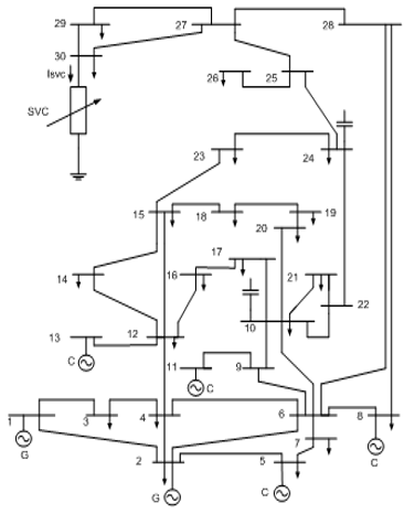
IEEE -30 bus sytem with one slack bus, 5-generator buses and 24 load buses as given in Figure 5
L-index value of all the load buses determined and tabulated in Table 5. From the L-index table it was observed that, 30th bus is having highest L-index value so it is the weak or critical bus. At normal loading and 200% increment in loading it is observed that the 30th bus was the weak bus.
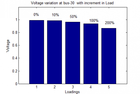
Increasing active and reactive load demands at 30-bus in between 10% to 200% from the normal value, all bus voltages tabulated in Table.6. It was observed that by increasing load at 30th bus not only voltage at that bus but also voltages at remain buses also changed. At 200% increment of load from base load the voltage at bus-30 is 0.8707 pu. Which is undesirable.
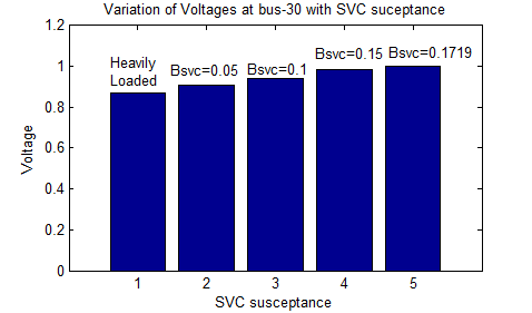
Since 30th bus is the weak bus location of SVC facts controller is 30th bus as given in Figure 5. When the system is under overloaded condition, SVC FACTS controller is connected and variation of voltages at all buses with respect to susceptance tabulated in Table 7 by varying
Figure 5. IEEE 30-bus System
Susceptance of SVC it was observed that not only volatage of 30th bus voltage increased but also voltage of all the buses increased. At exactly susceptance is equal to 1.1719 30th bus voltage reached to 1 pu.
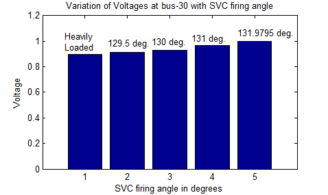
Variation of voltages at all buses by varying firing angle tabulated in Table 8.
Table 5. L-index values of IEEE-30 bus sytem
|
S.No |
Normal Loading |
|||
|
Bus No. |
L-Index |
Bus No. |
L-Index |
|
|
1 |
30 |
2.2146 |
16 |
0.1112 |
|
2 |
29 |
0.1667 |
17 |
0.1049 |
|
3 |
26 |
0.1392 |
15 |
0.0814 |
|
4 |
24 |
0.1333 |
14 |
0.0812 |
|
5 |
19 |
0.127 |
10 |
0.0805 |
|
6 |
20 |
0.1265 |
12 |
0.0703 |
|
7 |
25 |
0.1263 |
28 |
0.0666 |
|
8 |
23 |
0.1255 |
3 |
0.0634 |
|
9 |
21 |
0.1254 |
9 |
0.0522 |
|
10 |
27 |
0.1238 |
4 |
0.0384 |
|
11 |
18 |
0.1232 |
7 |
0.0375 |
|
12 |
22 |
0.1176 |
6 |
0.0133 |
Figure 6. Voltage Varition with incresed load demand
Table 6. Voltage variations with increment in load demand at load buses
|
Load Bus No. |
%Change in load Demand |
Load Bus No. |
%Change in load Demand |
||||||
|
0% |
10% |
50% |
200% |
0% |
10% |
50% |
200% |
||
|
3 |
1.0215 |
1.0214 |
1.0178 |
1.015 |
19 |
1.0253 |
1.0251 |
1.0225 |
1.0182 |
|
4 |
1.0129 |
1.0127 |
1.0084 |
1.0053 |
20 |
1.0293 |
1.0291 |
1.0265 |
1.0223 |
|
6 |
1.0121 |
1.0119 |
1.0082 |
1.005 |
21 |
1.0321 |
1.0319 |
1.029 |
1.0234 |
|
7 |
1.0034 |
1.0034 |
0.997 |
0.995 |
22 |
1.0327 |
1.0324 |
1.0295 |
1.0235 |
|
9 |
1.051 |
1.0509 |
1.0486 |
1.0457 |
23 |
1.0272 |
1.0269 |
1.0237 |
1.0156 |
|
10 |
1.0444 |
1.0442 |
1.0416 |
1.0375 |
24 |
1.0216 |
1.021 |
1.0168 |
1.004 |
|
12 |
1.0574 |
1.0573 |
1.0554 |
1.0531 |
25 |
1.0189 |
1.0176 |
1.0098 |
0.9799 |
|
14 |
1.0424 |
1.0423 |
1.0402 |
1.0371 |
26 |
1.0012 |
0.9999 |
0.992 |
0.9615 |
|
15 |
1.0379 |
1.0376 |
1.0352 |
1.0308 |
27 |
0.0257 |
1.024 |
1.0142 |
0.9747 |
|
16 |
1.0447 |
1.0445 |
1.0423 |
1.0392 |
28 |
1.0107 |
1.0103 |
1.0063 |
0.9979 |
|
17 |
1.0391 |
1.039 |
1.0365 |
1.0326 |
29 |
1.0059 |
1.0028 |
0.9867 |
0.918 |
|
18 |
1.0279 |
1.0278 |
1.0253 |
1.0209 |
30 |
0.9945 |
0.989 |
0.9675 |
0.8707 |
Table7. Variation of Voltages with SVC susceptance at load buses
|
Bus No. |
Heavily loaded (200%) |
Variation of Bus Voltages with Bsvc |
Bus No. 0.1 |
Heavily loaded (200%) |
Variation of Bus Voltages with Bsvc |
||||
|
0.1 |
0.15 |
1.1719 |
0.1 |
0.15 |
1.1719 |
||||
|
2 |
1.033 |
1.033 |
1.033 |
1.033 |
19 |
1.0182 |
1.0221 |
1.0242 |
1.0251 |
|
4 |
1.003 |
1.0066 |
1.0072 |
1.0075 |
20 |
1.0223 |
1.0261 |
1.0282 |
1.0292 |
|
6 |
1.005 |
1.0065 |
1.0073 |
1.0077 |
21 |
1.0234 |
1.0285 |
1.0313 |
1.0326 |
|
7 |
0.995 |
0.996 |
0.9964 |
0.9967 |
22 |
1.0235 |
1.0289 |
1.0319 |
1.0333 |
|
9 |
1.0457 |
1.048 |
1.0492 |
1.0498 |
23 |
1.0156 |
1.0221 |
1.0257 |
1.0273 |
|
10 |
1.0375 |
1.0414 |
1.0435 |
1.0445 |
24 |
1.004 |
1.0144 |
1.02 |
1.0227 |
|
12 |
1.0531 |
1.0552 |
1.0563 |
1.0568 |
25 |
0.9799 |
1.0038 |
1.0168 |
1.0228 |
|
14 |
1.0372 |
1.04 |
1.0415 |
1.0422 |
26 |
0.9615 |
0.9859 |
0.9991 |
1.0052 |
|
15 |
1.0308 |
1.0344 |
1.0364 |
1.0373 |
27 |
0.9747 |
1.0067 |
1.0242 |
1.0323 |
|
16 |
1.0392 |
1.042 |
1.0436 |
1.0443 |
28 |
0.9979 |
1.0023 |
1.0046 |
1.0057 |
|
17 |
1.0326 |
1.0362 |
1.0382 |
1.0391 |
29 |
0.918 |
0.9692 |
0.9971 |
1.0099 |
|
18 |
1.0209 |
1.0247 |
1.0267 |
1.0277 |
30 |
0.8707 |
0.9427 |
0.982 |
1 |
Table 8. Variation of voltages with firing angle at load buses
|
Bus No. |
Heavily loaded (200%) |
Variation of Bus voltages with asvc |
Bus No.
|
Heavily loaded (200%) |
Variation of Bus voltages with asvc |
||||
|
130° |
131° |
131.9795° |
130° |
131° |
131.9795° |
||||
|
3 |
1.015 |
1.0129 |
1.0134 |
1.0139 |
19 |
1.0182 |
1.0188 |
1.0206 |
1.0225 |
|
4 |
1.0053 |
1.0028 |
1.0034 |
1.004 |
20 |
1.0223 |
1.0227 |
1.0246 |
1.0265 |
|
6 |
1.005 |
1.0008 |
1.0015 |
1.0022 |
21 |
1.0234 |
1.0247 |
1.0272 |
1.0297 |
|
7 |
0.995 |
0.9926 |
0.993 |
0.9934 |
22 |
1.0235 |
1.0251 |
1.0277 |
1.0304 |
|
9 |
1.0457 |
1.0447 |
1.0458 |
1.047 |
23 |
1.0156 |
1.0186 |
1.0217 |
1.0249 |
|
10 |
1.0375 |
1.0378 |
1.0397 |
1.0415 |
24 |
1.004 |
1.0098 |
1.0148 |
1.0198 |
|
12 |
1.0531 |
1.053 |
1.054 |
1.0549 |
25 |
0.9799 |
0.9968 |
1.0083 |
1.0198 |
|
14 |
1.0371 |
1.0375 |
1.0388 |
1.0402 |
26 |
0.9615 |
0.9787 |
0.9904 |
1.0022 |
|
15 |
1.0308 |
1.0317 |
1.0334 |
1.0352 |
27 |
0.9747 |
0.9983 |
1.0137 |
1.0292 |
|
16 |
1.0392 |
1.0392 |
1.0406 |
1.042 |
28 |
0.9979 |
0.9954 |
0.9975 |
0.9995 |
|
17 |
1.0326 |
1.0329 |
1.0346 |
1.0363 |
29 |
0.918 |
0.9589 |
0.9835 |
1.0082 |
|
18 |
1.0209 |
1.0216 |
1.0234 |
1.0252 |
30 |
0.8707 |
0.9305 |
0.9651 |
1 |
Figure 7. Variation of Voltages with SVC susceptance
Figure 8. Variation of Voltages with SVC firing angle
Figure 9. Voltage variation at all buses under normal and heavily loaded case
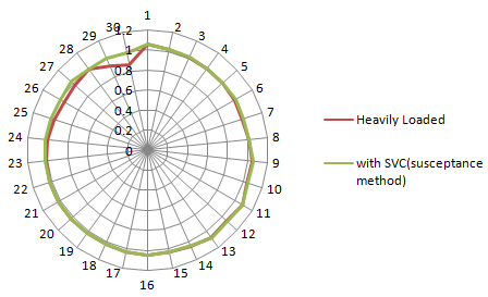
Figure 10. Variation of all bus voltages under hevily loaded and SVC with susceptance model
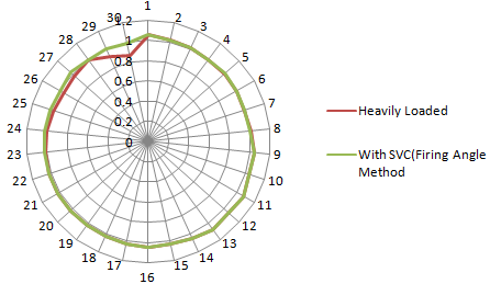
Figure 11. Variation of all bus voltages under heavily loaded and SVC with firing angle model
It was observed that when the system is under over loaded condition there will be voltage drop from the reference level which is undesirable in the system. SVC is the Shunt FACTS controller to support the voltage profile when there is a disturbance. To determine optimal location of FACTS controller L-index method is used. According to this method it was identified that 5th bus in standard IEEE 5-bus system, 30th bus in IEEE 30-bus system are weak buses. At these weak buses SVC FACTS controller is placed. Suceptance and Firing angle methods are considered. SVC has been providing good control over the bus voltage when there is disturbances such as over loading.
[1] Bujal, N.R., Hasan, A.E., Sulaiman, M. (2014). Analysis of voltage stability problems in power system. 4th International Conference on Engineering Technology and Technopreneuship(ICE2T), 27-29. https://doi.org/10.1109/ICE2T.2014.7006262
[2] Gupta, V.K., Kumar, S., Bhattacharyya, B. (2014). Enhancement of Power System Loadability with FACTS Devices. The Institution of Engineers (India), 95(2): 113–120. https://doi.org/10.1007/s40031-014-0085-0
[3] Dike, D.O., Mahajan, S.M. (2015). Voltage stability index based reactive power compensation scheme. Electrical Power and Energy System; 73: 734-742. https://doi.org/10.1016/j.ijepes.2015.04.016
[4] Saadat, H. (1999). Power System Analysis, McGraw-Hill Series in Electrical Computer Engineering.
[5] Perez, H.A., Ache, E., Esquivel, C.R.F. (2000). Advanced SVC Models for the Newton Raphson load flow and Newton optimal power flow studies. IEEE Transactions on the power systems, 15(1): 129-136. https://doi.org/10.1109/59.852111
[6] Huang, H.L., Kong, Y. (2008). The Analysis on the L-index based Optimal Power Flow Considering Voltage Stability Constraints. WSEAS Transactions on Systems, 7(11): 1300-1309.
[7] London, S.P., Rodriguez, L.F., Oliver, G. (2014). A simplified voltage stability index(SVSI). Electrical Power and Energy System; 63: 806-813. http://dx.doi.org/10.1016/j.ijepes.2014.06.044
[8] Abedelatti, A.E., Hashim, H., Abidin, I.Z., Sie, A.W.H., Nasional, U.T., Mara, T. (2015). Weakest Bus Based on Voltage Indices and Loadability, 8–9. http://dspace.uniten.edu.my/jspui/handle/123456789/10203
[9] Acha, E., Agelidis, V.G. (2006). Power Electronic Control in Electrical Systems, Newness.
[10] Lahacani, N.A., Mendil, B. (2008). Modeling and Simulation of the SVC for Power System Flow Studies. Leonardo Journal of Sciences, 153-170.
[11] Hernandez, A., Rodriguez, M.A., Torres, E., Eguia, P. (2013). A Review and Comparison of FACTS Optimal Placement for Solving Transmission System Issues. Renewable Energy and Power Quality Journal (RE&PQJ), (11). https://doi.org/10.24084/repqj11.435
[12] Thukaram, D., Lomi, A. (2000). Selection of Static VAR Compensator Location and Size for System Voltage Stability Improvements. Electrical Power System Research, 54: 139-150. https://doi.org/10.1016/S0378-7796(99)00082-6
[13] Suman, M., Rao, M.V.G., Rao, P.V.R. (2018). Enhancement of voltage stability using optimally sited static VAR compensator with three phase fault. Journal of Research in Dynamical & Control systems, 10(3): 95-106.
[14] Hassen, M.O., Cheng, S.J., Zakaria, Z.A. (2009). Steady State Modelling of SVC and TCSC for Power Flow Analysis. the international multi conference of engineering and computer scientists Proceeding, 2: 1443-1448.
[15] Kowsalya, M., Ray, K.K., Kotheri, D.P. (2009). Positioning of SVC and STATCOM in a Long Transmission Line. International journal of Recent Trends in Engineering, 2(5).