Robust Adaptive Control of Dual Star Asynchronous Machine by Reference Model Based on Landau Stability Theorem

The parameters of the machine generally depend on the operating point and vary with either the temperature (resistors) or the magnetic state of the machine (inductors), besides the load can be variable. That poses a problem of design of the control systems in the presence of uncertainties on the model of the process to be controlled in this situation. Indeed, automation engineers offer adaptive control. Thus, this command is established by sets of techniques used for the real-time automatic adjustment of the controllers of the control loops and this in order to achieve or maintain a certain level of performance when the parameters of the process to be controlled are unknown or vary in the time [1-3].

Recent developments indicate that robust adaptive control is provided by the enhancement performed in the closed loop process identification part. This leads to the calculation of a robust regulator in the presence of uncertainties on the model of the process. These uncertainties cover the variations of the parameters. There is therefore a strong interaction between robust adaptive control, closed-loop identification and robust controller calculation [3].

The rest of the article is organized as follows: Section 2 reviews the MRAC design. Then the closed-loop identification and its relation with the robust control are discussed in section 3. Section 4 presents a vector control strategy of the dual-star asynchronous machine with recalculate the RST regulator and explains the link with the MRAC adaptive control, then deduce a robust control law. Section 5 presents the simulation of the machine and testing the robustness of the regulators.

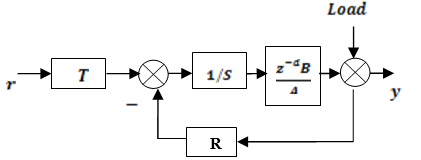
As discussed in the introduction about the strong iterative between robust control and closed-loop identification and adaptive control, this iterative forces the automation engineer to create new identification algorithms [6-7]. New algorithms were developed in the nineties in the context of the iterative approach for closed-loop identification and recalculate the regulator. In fact, closed-loop identification can not be dissociated from the regulator and robustness considerations. The basic scheme of a digital control loop is shown in Figure 2, the model of the machine is characterized by a transfer operator (where $z^{-1}$ is the unit delay operator). 

$\mathrm{G}\left(\mathrm{z}^{-1}\right)=\mathrm{z}^{-\mathrm{d}} \frac{\mathrm{B}\left(\mathrm{z}^{-1}\right)}{\mathrm{A}\left(\mathrm{z}^{-1}\right)}(\text {Karimi Model })$

$\begin{aligned} \mathrm{B}\left(\mathrm{z}^{-1}\right)=& \mathrm{b}_{1} * \mathrm{z}^{-1}+\cdots \mathrm{b}_{\mathrm{n}_{\mathrm{B}}} \mathrm{z}^{-\mathrm{n}_{\mathrm{p}}} =\mathrm{z}^{-1} \mathrm{B}^{*}\left(\mathrm{z}^{-1}\right) \end{aligned}$         (1)

$\begin{aligned} \mathrm{A}\left(\mathrm{z}^{-1}\right)=& 1+\mathrm{a}_{1} * \mathrm{z}^{-1}+\cdots \mathrm{a}_{\mathrm{n}_{\mathrm{A}}} \mathrm{z}^{-\mathrm{n}_{\mathrm{A}}} =1+\mathrm{z}^{-1} \mathrm{A}^{*}\left(\mathrm{z}^{-1}\right) \end{aligned}$

with d the deley.

2.png

Figure 2. Closed loop system with R-S-T controller

The closed-loop system uses a digital R-S-T controller. The output of the machine (process), in closed loop, is given by:

$\mathrm{y}(\mathrm{t}+1)=-\mathrm{A}^{*} \mathrm{y}(\mathrm{t})+\mathrm{B}^{*} \mathrm{u}(\mathrm{t}-\mathrm{d})+\mathrm{A} * \xi(\mathrm{t}+1)=\theta^{\mathrm{T}} \varphi(\mathrm{t})+\mathrm{A} \xi(\mathrm{t}+1)$         (2)

with u(t) is the input of the process, y(t) is the output of the process, $\xi(t)$ is the disturbance (Load) and:

$\theta^{\mathrm{T}}=\left[\mathrm{a}_{1} \ldots \mathrm{a}_{\mathrm{n_A}} \mathrm{b}_{1} \ldots \mathrm{b}_{\mathrm{n}_{\mathrm{b}}}\right]$        (3)

$\varphi^{\mathrm{T}}=\left[-\mathrm{y}(\mathrm{t}) \ldots-\mathrm{y}\left(\mathrm{t}-\mathrm{n}_{\mathrm{A}}+1\right) \mathrm{u}(\mathrm{t}-\mathrm{d}) \ldots \mathrm{u}\left(\mathrm{t}-\mathrm{n}_{\mathrm{B}}+1-d)]\right.\right.$            (4)

$u(t)=-\frac{R\left(z^{-1}\right)}{S\left(z^{-1}\right)} y(t)+r_{u}^{\prime}(t)$            (5)

with $r_{\mathrm{u}}^{\prime}$ is the equivalent external excitation superimposed on the output of the regulator. In general:

$r_{u}^{\prime}=\frac{T\left(z^{-1}\right)}{S\left(z^{-1}\right)} r+r_{u}$              (6)

where $r$ is the reference signal and $r_{u}$ is an external signal added to the output of the regulator. In Gonzalez [7], robustness and closed-loop identification for regulator design is achieved by the sensitivity functions as follows:

The disturbance-output sensitivity function is given by:

$S_{\mathrm{yp}}\left(\mathrm{z}^{-1}\right)=\frac{\mathrm{A}\left(\mathrm{z}^{-1}\right) \mathrm{S}\left(\mathrm{z}^{-1}\right)}{\mathrm{C}\left(\mathrm{z}^{-1}\right)}$      (7)

The disturbance-input sensitivity function is given by:

$S_{\mathrm{up}}\left(\mathrm{z}^{-1}\right)=-\frac{\mathrm{A}\left(\mathrm{z}^{-1}\right) \mathrm{R}\left(\mathrm{z}^{-1}\right)}{\mathrm{C}\left(\mathrm{z}^{-1}\right)}$            (8)

And $\mathrm{C}\left(\mathrm{z}^{-1}\right)$ is the characteristic polynomial of the closed loop whose roots are the poles of the closed loop:

$\mathrm{C}\left(\mathrm{z}^{-1}\right)=\mathrm{A}\left(\mathrm{z}^{-1}\right) \mathrm{S}\left(\mathrm{z}^{-1}\right)+\mathrm{z}^{-\mathrm{d}} \mathrm{B}\left(\mathrm{z}^{-1}\right) \mathrm{R}\left(\mathrm{z}^{-1}\right)$            (9)

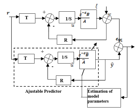
Techniques to combine the achievement of nominal performance with the calibration of sensitivity functions have been developed and applied in practice [4,8], where the fundamental purpose of closed-loop identification is to obtain a process model that leads to a better prediction of the behavior of the real closed loop. This principle is illustrated in Fig.3 where the parametric adaptation algorithm will modify the model parameters to minimize the closed-loop output error. By following this approach consisting of algorithm families called "Closed loop output error (CLOE)" it was developed by Gang et al. [9-10], their common feature is the structure of the adjustable predicator shown in Figure 3 and given by: $\hat{\mathrm{y}}(\mathrm{t}+1)=\hat{\theta}^{\mathrm{T}}(\mathrm{t}) \varphi(\mathrm{t})$.

3.png

Figure 3. Identification by the method of closed loop output error

$\hat{\theta}(t)=\left[\hat{a}_{1}(t) \ldots \hat{a}_{n_{A}}(t) \hat{b}_{1}(t) \ldots \hat{b}_{n_{B}}(t)\right]$,

$\varphi^{T}(t)=\left[-\hat{y}(t) \ldots-\hat{y}\left(t-n_{A}+1\right) \hat{u}(t-d) \ldots \hat{u}(t-\right.\left.\left.n_{B}+1-d\right)\right]$

$\hat{y}(t)=\hat{\theta}^{T}(t) \varphi(t-1)$

$\hat{u}(\mathrm{t})=-\frac{\mathrm{R}\left(\mathrm{z}^{-1}\right)}{\mathrm{S}\left(\mathrm{z}^{-1}\right)} \hat{\mathrm{y}}(\mathrm{t})+\mathrm{r}_{\mathrm{u}}^{\prime}(\mathrm{t}), \mathrm{r}_{\mathrm{u}}^{\prime}=\frac{\mathrm{T}\left(\mathrm{z}^{-1}\right)}{\mathrm{S}\left(\mathrm{z}^{-1}\right)} \mathrm{r}+\mathrm{r}_{\mathrm{u}}$.

The output error in closed loop is given by:

$\epsilon(t+1)=y(t+1)-\hat{y}(t+1)=\frac{s}{p}(\theta(t)-\hat{\theta}(t+1))^{T} \varphi(t)+\omega^{\prime}(t+1)$,

with: $\omega^{\prime}(\mathrm{t}+1)=\frac{\mathrm{AS}}{\mathrm{P}} \omega(\mathrm{t}+1)=\mathrm{S}_{\mathrm{yp}} \omega(\mathrm{t}+1)$.

According to [15], all algorithms use the following parametric adaptation algorithm:

$\hat{\theta}(\mathrm{t}+1)=\hat{\theta}(\mathrm{t})+\mathrm{F}(\mathrm{t}) \varphi(\mathrm{t}) \epsilon_{\mathrm{cL}}(\mathrm{t}+1)$       (10)

$\mathrm{F}(\mathrm{t}+1)^{-1}=\lambda_{1}(\mathrm{t}) \mathrm{F}^{-1}+\lambda_{2}(\mathrm{t}) \varphi(\mathrm{t}) \varphi(\mathrm{t})^{\mathrm{T}}$      (11)

$0<\lambda_{1} \leq 1 ; 0 \leq \lambda_{2}<2$     (12)

$\epsilon_{\mathrm{CL}}(\mathrm{t}+1)=\mathrm{y}(\mathrm{t}+1)-\hat{\mathrm{y}}(\mathrm{t}+1)\quad=\frac{\mathrm{y}(\mathrm{t}+1)-\widehat{\mathrm{y}}(\mathrm{t}+1)}{1+\varphi^{\mathrm{T}}(\mathrm{t}) \mathrm{F}(\mathrm{t}) \varphi(\mathrm{t})}$        (13)

The difficulty in controlling a dual stator asynchronous machine lies in the fact that there is a strong coupling between the input and output variables and the internal variables of the machine such as flux, torque and speed [3,11]. Conventional control methods such as torque control by frequency slip and flux by the ratio of voltage to frequency, this type of control can not ensure significant dynamic performance [3,12], the development of electronics in the use of static and semi-conductive converters, allowed the application of new control algorithms such as the control identical to that of the MCC.

Vector control is based on the decoupling of flux and torque in AC machines [1]. The vector control leads to high industrial performance of asynchronous drives if the rotor flow coincides with the axis (d) of the reference linked to the rotating field. And after the rotor flow orientation by: $\varphi_{\mathrm{rd}}=\varphi_{\mathrm{d}}, \varphi_{\mathrm{rq}}=0$ so:

$\mathrm{C}_{\mathrm{em}}=\mathrm{p} \frac{\mathrm{L}_{\mathrm{m}}}{\mathrm{L}_{\mathrm{m}}+\mathrm{L}_{\mathrm{r}}}\left(\mathrm{i}_{\mathrm{qs} 1}+\mathrm{i}_{\mathrm{qs} 2}\right) \varphi_{\mathrm{r}}$         (16)

The main objective according to Hellali et al. [1,13], is to produce reference voltages for the static voltage converters supplying the DSIM. Note $X^{*}$ for reference quantities (torque, flux, voltages and currents). The application of the orientation of the rotor flux on the system of equations of the machine leads to [5-20-1]: $T_{r}=\frac{L_{r}}{R_{r}}, \omega_{s}^{*}=\omega_{s r}^{*}+\omega_{r}, \omega_{s r}^{*}$

$\varphi_{r}=L_{m}\left(I_{s 1 d}+I_{s 2 d}\right)$        (17)

$C_{e m}^{*}=P \frac{L_{m}}{L_{m}+L_{r}} \varphi_{r}^{*}\left(I_{s q 1}+I_{s q 2}\right)$       (18)

$\omega_{s r}^{*}=\frac{R_{r} L_{m}}{\left(L_{m}+L_{r}\right) \varphi_{r}^{*}}\left(I_{s q 1}^{*}+I_{s q 2}^{*}\right)$             (19)

$V_{s 1 d}^{*}=R_{s 1} I_{s 1 d}+L_{s 1} \frac{d}{d t} I_{d s 1}-\omega_{s}^{*}\left(L_{s 1} I_{s 1 q}+\right.\left.T_{r} \varphi_{r}^{*} \omega_{s r}^{*}\right)$         (20)   

$\begin{aligned} V_{s 2 d}^{*}=R_{s 2} I_{s 2 d}+& L_{s 1} \frac{d}{d t} I_{d s 2} -\omega_{s}^{*}\left(L_{s 1} I_{s 2 q}+T_{r} \varphi_{r}^{*} \omega_{s r}^{*}\right) \end{aligned}$       (21)

$\mathrm{V}_{\mathrm{s} 1 \mathrm{q}}^{*}=\mathrm{R}_{\mathrm{s} 1} \mathrm{I}_{\mathrm{s} 1 \mathrm{q}}+\mathrm{L}_{\mathrm{s} 1} \frac{\mathrm{d}}{\mathrm{dt}} \mathrm{I}_{\mathrm{qs} 1}+\omega_{\mathrm{s}}^{*}\left(\mathrm{L}_{\mathrm{s} 1} \mathrm{I}_{\mathrm{s} 1 \mathrm{d}}+\varphi_{\mathrm{r}}^{*}\right)$     (22)

$\mathrm{V}_{\mathrm{s} 2 \mathrm{q}}^{*}=\mathrm{R}_{\mathrm{s} 2} I_{s 2 q}+L_{s 2} \frac{d}{d t} I_{q s 2}+\omega_{s}^{*}\left(L_{s 2} I_{s 2 d}+\varphi_{r}^{*}\right)$      (23)

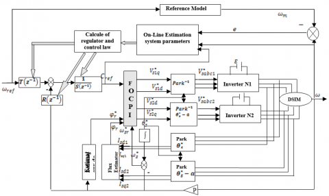
The current regulators have been made by the classical PI regulator in order to ensure a better robustness with respect to internal or external disturbances. Figure 4 shows the robust MRAC speed control scheme where the machine associated with two identical voltage inverters.

4.png

Figure 4. Scheme of the decoupled control by flux orientation applied to the DSIM

5.1 Simulation results

The robust regulator developed in Section 3 is evaluated in simulation, using a 4.5 kW double-stator asynchronous motor, whose characteristics are summarized in APPENDIX B, fed by two identical inverters. The robust MRAC regulator performance is illustrated by forcing the machine to operate under different conditions: forward and reverse speed, loaded and unloaded motor. For robust identification, the parameters of the regulators are given the following values which have proved to be suitable: $\theta^{\mathrm{T}}(0)=[0 \cdots 0.01]$, so: $\omega(\mathrm{t})=\mathrm{z}^{-2} \frac{\mathrm{b}}{1+\mathrm{az}^{-1}} \mathrm{C}_{\mathrm{em}}^{*}(\mathrm{t})$.

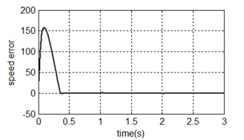
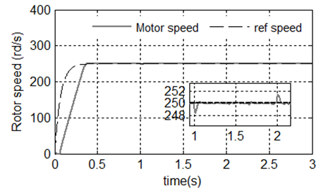
According to the Youb et al. [13-14], to avoid the convergence toward zero of adaptation gain, we pose: $\lambda_{1}(\mathrm{k})=1$ and, $0<\lambda_{2}(\mathrm{k})<2$, with the initial adaptation gain is $\mathrm{F}(0)=\mathrm{I}_{2}, \mathrm{Kp}=100, \mathrm{ki}=50$ Figure.5 shows that robust MRAC controllers have ensured a perfect speed reference tracking since the rotor speed reaches the reference speed after t = 0.45s and has an overshoot of less than 1%. The application of the load generates a weak attenuation of the speed during a short time 0.05s then it resumes the value of speed of reference 2860 rpm (one applies a load of 14N.m to the (1:2) s), The two rotor axis component d and q shown in Figure 7, according to the values imposed in fully established regime and regardless of the applied load. So we say that the decoupling of FOC is perfect.

Figure 8.a shows that the electromagnetic torque has a damped sinusoidal shape in the transient regime, with a starting value of 75N.m. When the speed reaches the setpoint, the torque oscillates zero and after the insertion of the load, the electromagnetic torque compensates the load torque and friction.

In steady state the current iqs1 has the same pace as that of the electromagnetic torque therefore the speed regulation of the DSIM is similar to that of the MCC with separate excitation $\left(\mathrm{C}_{\mathrm{em}}=\mathrm{K} * \mathrm{I}\right)$, (Figure 8b). From the curve of the stator current Ias1, we see that its value at startup touches a peak value, and in the presence of the load (zoom), the current reaches a value max = 10A. The current is sinusoidal and has harmonics due to the two voltage inverters.

5.png

Figure 5. Simulation result of speed

6.png

Figure 6. Output error of Speed $\left(\omega_{\mathrm{r}}-\omega_{\mathrm{m}}\right)$

7.png

Figure 7. Rotor flux component d and q (phidr, phiqr)

8.png

Figure 8. Presentation of electromagnetic Torque, current (I_ds1 I_qs1) and stator current

5.2 Test de robustness

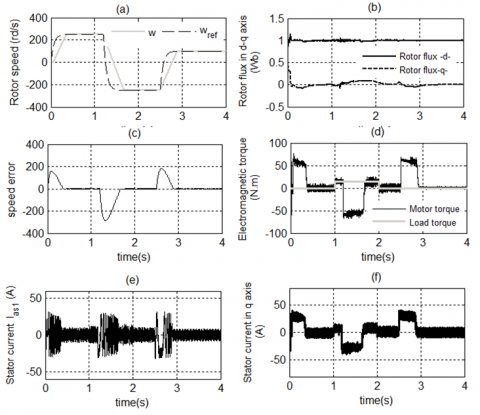
The robustness of a robust MRAC command is made by the behavior test of the regulation with respect to the variations of the parameters of the DSIM. Since the operation of electrical machines is sensitive to variations in the rotor time constant. We will increase the rotor resistance Rr of the DSIM compared to its nominal value Rr=2* Rn at t=[0.8-1.5] s. With the reversal of the load speed, Cr=14N.m applied to t=[1-2].

During the transient regime and before the reversal of the speed (from t = 0s to 1.2s), the curves  evolve in a way identical to that observed previously (Figure 8.a, b, c), from t = 1.2s, the speed reverses and reaches its negative setpoint after t = 0.48s without any overtaking. This creates an increase in current Ias1 which is equal to the value recorded during start-up, which stabilizes after 0.48s, to give back to the shape of the steady state, the electromagnetic torque reaches (-55Nm) at moment of the inversion of the speed, which stabilizes at its negative setpoint (-2500 rpm), the quadrature current Iqs1 progresses in a manner consistent with the electromagnetic torque, the curves of the rotor flux components observe a slight variation during the reversal of the speed. The robustness test shows the insensitivity of the speed control by the robust MRAC regulator to the parametric variations due to the increase of Rr to [0.8-1.5] s of the machine.

Nomenclature of the parameters DSIM model