Herizi Abdelghafour | Bouguerra Abderrahmen | Zeghlache Samir | Rouabhi Riyadh
OPEN ACCESS
In this paper, we present a new sliding mode control strategy applied to the doubly fed induction machine, this control combines sliding mode and type-2 fuzzy logic to find robust control. The proposed control kept the part of the equivalent control by sliding mode and will change the part of the switching by a type-2 fuzzy controller has an input is the error between the measured value and the reference value. In this command we apply the orientation of the stator flux to have the decoupling between the flux and the current. The results obtained in simulation show the effectiveness of this command.
sliding mode, Type-2 fuzzy logic, doubly fed induction machine, stator flux orientation, hybrid control, robustness
Currently, AC motors are more used because these machines are characterized by their robustness and longevity but internal structures and control strategies more complex.
Nowadays, several works have been directed towards the study of the doubly-fed induction machine (DFIM) [1-3], it is a three-phase asynchronous machine with a wound rotor that can be powered by two voltage sources [4], one to the stator and the other to the rotor. For variable speed operation, a PWM (Pulse Width Modulation) inverter must be inserted between the machine and the network.
Thanks to the recent technological evolution of power electronics and the emergence of modern control techniques, the DFIM presents an ideal solution for high performance and variable speed drives [5]. The interest of such a machine is ensured operation at a very low speed. The potential application of the MADA has been a topic of research over the last decade.
Despite all the advantages of the DFIM: low manufacturing cost, relatively simple construction, overload support, higher rotation speed and no need for permanent maintenance. The control of this machine is more complex because of the coupling existing between their different state variables (non-linear and strongly coupled) and a large number of control variables [6, 7].
The control techniques classics (for example PI and PID controllers) require a perfect knowledge of the system model to be adjusted. These approaches lead to control laws whose performance is strongly related to the fidelity of the dynamic model used to describe the system behavior. Modeling errors or variations in system parameters can affect the performance of the adjustment as they occur directly in the calculation of the control.
Among several types of modern controls that have attracted the intention of many researchers in recent years, the sliding mode control. Recent interest in this control is primarily the availability of high switching frequency switches and high performance microprocessors.
The algorithm of sliding mode control is classified in Variable Structure control System (VSS). This technique is based on the principle that it is easier to 1st order system than to nth order system, whether linear or not. The principle of this type of system with variable structure is to bring, whatever the initial conditions, the representative point of the evolution of the system on the surface of the phase space (representing a set of relations between the state variables). The considered surface is then designated as a sliding or switching surface. The resulting dynamic behavior, called the ideal sliding regime, is completely determined by the parameters and equations defining the surface [8].
The advantage of obtaining such a behavior is twofold: on the one hand, there is a reduction in the order of the system, and on the other hand, the sliding regime insensitive to disturbances occurring in the same directions as the inputs (matching disturbances).
The sliding mode control is largely proven to be effective through the reported theoretical studies, these main fields of application are robotics [9, 10] and electric motors [11]. The advantage of this control is to ensure the robustness of uncertain and disturbed systems by mitigating the effects of external disturbances to the desired level [12, 13]. However, these performances are obtained at the cost of certain disadvantages:
A phenomenon of chattering or chatter caused by the discontinuous part of this command and which can have a detrimental effect on the actuators,
The system is constantly subjected to high control to ensure its convergence to the desired state and this undesirable.
We propose in this work to terminate these problems a command that combines the sliding mode and type-2 fuzzy logic to obtain a robust control. This command is named type 2 fuzzy sliding mode control, which consists of replacing the switching function in the sliding mode control with a type 2 fuzzy controller. An input is the error between the measured value and the reference value. In order to test its efficiency and robustness, the latter is applied to the control of the doubly-fed induction machine, taking into account the parametric variations of its dynamic model.
In this paper, mathematical model of the DFIM in (d, q) reference is presented followed by the orientation of the stator flux. Then, the theoretical study on type 2 fuzzy logic. In the fourth section, we synthesize the law of the control by the sliding mode and type-2 fuzzy of the MADA, following the strategy of the command by the sliding mode which allows an independent control the output state variables. Finally, the robustness tests of the control of the machine will be carried out. The simulations will be presented under Matlab/Simulink.
The machine used is supposed to have sinusoidal distribution, symmetrical and unsaturated. It is supplied with voltage through a PWM inverter. In a reference linked to the rotating field (d, q), the electrical equations of the DFIM write in the form:
$\left\{\begin{array}{l}V_{s d}=R_{s} I_{s d}+\frac{d \varphi_{s d}}{d t}-\omega_{s} \varphi_{s q} \\ V_{s q}=R_{s} I_{s q}+\frac{d \varphi_{s q}}{d t}+\omega_{s} \varphi_{s d} \\ V_{r d}=R_{r} I_{r d}+\frac{d \varphi_{r d}}{d t}-\left(\omega_{s}-\omega_{r}\right) \varphi_{r q} \\ V_{r q}=R_{r} I_{r q}+\frac{d \varphi_{r q}}{d t}+\left(\omega_{s}-\omega_{r}\right) \varphi_{r d}\end{array}\right.$ (1)
where:
$\omega_{r}=\omega_{s}-P . \Omega$
The magnetic equations of the DFIM can be written:
$\left\{\begin{array}{l}\varphi_{s d}=L_{s} I_{s d}+M . I_{r d} \\ \varphi_{s q}=L_{s} I_{s q}+M . I_{r q} \\ \varphi_{r d}=L_{r} I_{r d}+M . I_{s d} \\ \varphi_{r q}=L_{r} I_{r q}+M . I_{s q}\end{array}\right.$ (2)
$L_{s}=l_{s}-M_{s}$ and $L_{r}=l_{r}-M_{r}$: cyclic inductances of a stator and rotor phase;
$\left[l_{s}\right]$ and $\left[l_{r}\right]$: own inductances of a stator and rotor phase;
$M_{s}$ and $M_{r}$: mutual inductances between two phases respectively stator and rotor;
M: maximum mutual inductance between a stator and rotor phase (the axes of the two phases coincide).
The expression of the electromagnetic torque of the DFIM according to the stator flows and currents is written as follows:
$C_{e m}=P \frac{M}{L_{\mathrm{s}}}\left(\varphi_{s q} I_{r d}-\varphi_{s d} I_{r q}\right)$ (3)
with P: number of pairs of DFIM poles.
The model of the doubly-fed induction machine can be written in matrix form as follows [5]:
$\dot{X}=A X+B U$ (4)
where:
$X=\left[\begin{array}{lllllll}\varphi_{s d} & \varphi_{s q} & I_{r d} & I_{r q}\end{array}\right]^{T}$ and $U=\left[\begin{array}{llll}V_{s d} & V_{s q} & V_{r d} & V_{r q}\end{array}\right]^{T}$
$[A]=\left[\begin{array}{cccc}-\frac{1}{T_{s}} & \omega_{s} & \frac{M}{T_{s}} & 0 \\ -\omega_{s} & -\frac{1}{T_{s}} & 0 & \frac{M}{T_{s}} \\ \alpha & -\beta \omega & -\delta & \left(\omega_{s}-\omega\right) \\ \beta \omega & \alpha & -\left(\omega_{s}-\omega\right) & -\delta\end{array}\right]$
$[B]=\left[\begin{array}{cccc}1 & 0 & 0 & 0 \\ 0 & 1 & 0 & 0 \\ -\frac{M}{\sigma L_{s} L_{r}} & 0 & \frac{1}{\sigma L_{r}} & 0 \\ 0 & -\frac{M}{\sigma L_{s} L_{r}} & 0 & \frac{1}{\sigma L_{r}}\end{array}\right]$
with:
$\sigma=1-\frac{M^{2}}{L_{r} L_{s}} ; T_{r}=\frac{L_{r}}{R_{r}} ; T_{s}=\frac{L_{s}}{R_{s}} ; \alpha=\frac{M}{\sigma L_{r} L_{s} T_{s}} ; \beta=\frac{M}{\sigma L_{r} L_{s}} ; \delta=\frac{1}{\sigma}\left(\frac{1}{T_{r}}+\frac{M^{2}}{L_{s} T_{s} L_{r}}\right)$
The mechanical equation is of the following form:
$J \frac{d \Omega}{d t}=C_{e m}-C_{r}-f \Omega$ (5)
with:
$C_{e m}$ and $C_{r}$: the electromagnetic torque and the resisting torque (the mechanical load);
f and J: coefficient of friction and moment of inertia of the rotor shaft.
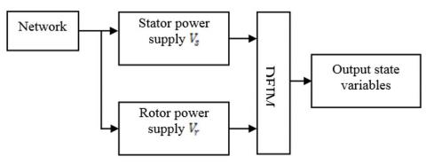
The synoptic diagram of a direct chain is given by the following figure:
Figure 1. Block diagram of a direct chain of DFIM
In our study, the frequency and the tension are constant. We can see, from relation (3), the strong coupling between flows and currents. Indeed, the electromagnetic torque is the cross product between the flows and the stator currents, which makes the control of the DFIM particularly difficult. In order to simplify the order, we approximate its model to that of the DC machine which has the advantage of having a natural decoupling between the flows and the currents. For this, we apply the flow orientation control which consists in aligning the stator flux $φ_s$ along the d axis of the rotating reference, (Figure 2), [14, 15]. We thus have: $\varphi_{s d}=\varphi_{s}$ and consequently $\varphi_{s q}=0$.
Figure 2. Stator flux orientation on the d axis
The electromagnetic torque of equation (3) is then written:
$C_{e m}=-P \frac{M}{L_{s}} \varphi_{s d} I_{r q}$ (6)
And the equation (2) of the flows becomes:
$\left\{\begin{array}{l}\varphi_{s d}=\varphi_{s}=L_{s} I_{s d}+M . I_{r d} \\ \varphi_{s q}=0=L_{s} I_{s q}+M . I_{r q}\end{array}\right.$ (7)
So: $\left\{\begin{array}{l}I_{s d}=\frac{1}{L_{s}}\left(\varphi_{s}-M I_{r d}\right) \\ I_{s q}=-\frac{1}{L_{s}} M I_{r q}\end{array}\right.$
If one takes the stator current in the axis of null, $I_{s d}=0$, realistic hypothesis for the machines of high power, the current and the tension in this axis are then in phase $V_{s}=V_{s q}$ and $I_{s}=I_{s q}$.
In this case, we get:
$\left\{\begin{array}{l}I_{r d}=\frac{\varphi_{s}}{M} \\ I_{r q}=-\frac{L_{s}}{P M \varphi_{s}} C_{e m}\end{array}\right.$ (8)
With the assumption of constant stator flux, we obtain the electric equations in the form:
$\left\{\begin{array}{l}V_{s d}=R_{s} I_{s d} \\ V_{s q}=R_{s} I_{s q}+\omega_{s} \varphi_{s d} \\ V_{r d}=R_{r} I_{r d}-\left(\omega_{s}-\omega_{r}\right) \varphi_{r q} \\ V_{r q}=R_{r} I_{r q}+\left(\omega_{s}-\omega_{r}\right) \varphi_{r d}\end{array}\right.$ (9)
In the principle of the orientation of the stator field, the model of the doubly-fed induction machine is written:
$\left\{\begin{array}{l}\frac{d \varphi_{s d}}{d t}=\frac{M}{T_{s}} I_{r d}-\frac{1}{T_{S}} \varphi_{s d}+V_{s d} \\ \frac{d \varphi_{s q}}{d t}=\frac{M}{T_{s}} I_{r q}-\omega_{s} \varphi_{s d}+V_{s q} \\ \frac{d I_{r d}}{d t}=-\delta I_{r d}+\left(\omega_{s}-\omega\right) I_{r q}+\alpha \varphi_{s d}-\frac{M}{\sigma L_{s} L_{r}} V_{s d}+\frac{1}{\sigma L_{r}} V_{r d} \\ \frac{d I_{r q}}{d t}=-\left(\omega_{s}-\omega\right) I_{r d}-\delta I_{r q}+\beta \omega \varphi_{s d}-\frac{M}{\sigma L_{s} L_{r}} V_{s q}+\frac{1}{\sigma L_{r}} V_{r q}\end{array}\right.$ (10)
The mechanical equation is written:
$\frac{d \Omega}{d t}=-\frac{1}{J}\left(P \frac{M}{L_{s}} \varphi_{s d} I_{r q}+f \Omega+C_{r}\right)$ (11)
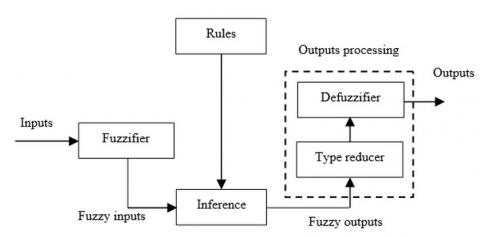
Type-1 and type-2 fuzzy logic are mainly similar. However, there exist two essential differences between them which are: the membership functions shape and the output processor. Indeed, an interval type-2 fuzzy controller is consisting of: a fuzzifier, an inference engine, a rules base, a type reduction and a defuzzyfier [16, 17].
3.1 Fuzzifier
The fuzzifier maps the crisp input vector $\left(e_{1}, e_{2}, \ldots, e_{n}\right)^{T}$ to a type-2 fuzzy system $\tilde{A}_{x},$ very similar to the procedure performed in a type-1 fuzzy logic system.
3.2 Rules
The general form of the $i^{t h}$ rule of the type-2 fuzzy logic system can be written as:
If $e_{1}$ is $\tilde{F}_{1}^{i}$ and $e_{2}$ is $\tilde{F}_{2}^{i}$ and $\ldots e_{n}$ is $\tilde{F}_{n}^{i},$ than
$y^{i}=\tilde{G}^{i} \quad i=1, \dots, M$ (12)
where:
$\tilde{F}_{j}^{i}$ represent the type- 2 fuzzy system of the input state $j$ of the $i^{t h}$ rule, $x_{1}, x_{2}, \ldots, x_{n}$ are the inputs, $\tilde{G}^{i}$ is the output of type-2 fuzzy system for the rule $i,$ and $M$ is the number of rules. As can be seen, the rule structure of type- 2 fuzzy logic system is similar to type-1 fuzzy logic system except that type-1 membership functions are replaced with their type-2 counterparts.
3.3 Inference Engine
In fuzzy system interval type- 2 using the minimum or product t-norms operations, the $i^{t h}$ activated rule $F^{i}\left(x_{1}, x_{2}, \ldots, x_{n}\right)$ gives us the interval that is determined by two extremes $\underline{f}^{i}\left(x_{1}, x_{2}, \ldots, x_{n}\right)$ and $\bar{f}^{i}\left(x_{1}, x_{2}, \ldots, x_{n}\right)[18]:$
$F^{i}\left(x_{1}, \ldots, x_{n}\right)=\left[\underline{f}^{i}\left(x_{1}, \ldots, x_{n}\right), \bar{f}^{i}\left(x_{1}, \ldots, x_{n}\right)\right] \equiv\left[\underline{f}^{i}, \bar{f}^{i}\right]$ (13)
With $\underline{f}^{i}$ and $\bar{f}^{i}$ are given as:
$\underline{f}^{i}=\underline{\mu}_{F_{1}^{i}}\left(x_{1}\right) \times \ldots \times \underline{\mu}_{F_{n}^{i}}\left(x_{n}\right)$
$\bar{f}^{i}=\bar{\mu}_{F_{1}^{i}}\left(x_{1}\right) \times \ldots \times \bar{\mu}_{F_{n}^{i}}\left(x_{n}\right)$ (14)
3.4 Type Reducer
After the rules are fired and inference is executed, the obtained type-2 fuzzy system resulting in type-1 fuzzy system is computed. In this part, the available methods to compute the centroid of type-2 fuzzy system using the extension principle [19] are discussed. The centroid of type-1 fuzzy system A is given by:
$C_{A}=\frac{\sum_{i=1}^{n} z_{i} w_{i}}{\sum_{i=1}^{n} w_{i}}$ (15)
where: $n$ represents the number of discretized domain $\operatorname{of} A, z_{i} \in R$ and $w_{i} \in[0,1]$.
If each $z_{i}$ and $w_{i}$ are replaced with a type- 1 fuzzy system, $Z_{i}$ and $W_{i},$ with associated membership functions of $\mu_{Z}\left(Z_{i}\right)$ and $\mu_{W}\left(W_{i}\right)$ respectively, by using the extension principle, the generalized centroid for type- 2 fuzzy system $\tilde{A}$ is given by:
$G C_{\tilde{A}}=\int_{z_{1} \in Z_{1}} \ldots \int_{z_{n} \in Z_{n}} \int_{w_{1} \in W_{1}} \ldots \int_{w_{n} \in W_{n}} \frac{T_{i=1}^{n} \mu_{Z}\left(Z_{i}\right) \times T_{i=1}^{n} \mu_{W}\left(W_{i}\right)}{\frac{\sum_{i=1}^{n} Z_{i} W_{i}}{\sum_{i=1}^{n} W_{i}}}$ (16)
T is a t-norm and$G C_{\tilde{A}}$is a type-1 fuzzy system. For an interval type-2 fuzzy system:
$G C_{\tilde{A}}=\left[y_{l}(x), y_{r}(x)\right]$
$=\int_{y^{1} \in\left[y_{l}^{1}, y_{r}^{1}\right]} \cdots \int_{y^{M} \in\left[y_{l}^{M}, y_{r}^{M}\right]} \int_{f^{1} \in\left[f^{1}, f^{1}\right]} \cdots \int_{f^{M} \in\left[\underline{f}^{M}, \bar{f}^{M}\right]} \frac{1}{\frac{\sum_{i=1}^{M} f^{i} y^{i}}{\sum_{i=1}^{M} f^{i}}}$ (17)
3.5 Defuzzifier
To get a crisp output from a type-1 fuzzy logic system, the type-reduced set must be defuzzied. The most common method to do this is to find the centroid of the type-reduced set. If the type-reduced set Y is discretized to n points, then the following expression gives the centroid of the type-reduced set as:
$Y(x)=\frac{\sum_{i=1}^{M} y^{i} \mu\left(y^{i}\right)}{\sum_{i=1}^{M} \mu\left(y^{i}\right)}$ (18)
We can compute the output using the iterative Karnik Mendel Algorithms [20, 21]. Therefore, the defuzzified output of an interval type-2 FLC is:
$Y(x)=\frac{y_{l}(x)+y_{r}(x)}{2}$ (19)
with:
$\left\{\begin{array}{l}y_{l}(x)=\frac{\sum_{i=1}^{M} f_{l}^{i} y_{l}^{i}}{\sum_{i=1}^{M} f_{l}^{i}} \\ y_{r}(x)=\frac{\sum_{i=1}^{M} f_{r}^{i} y_{r}^{i}}{\sum_{i=1}^{M} f_{r}^{i}}\end{array}\right.$ (20)
The structure of a fuzzy system Type-2 is shown in the figure 3. It is similar to the structure of a fuzzy system Type-1.
Figure 3. Structure of type-2 fuzzy logic system [22, 23]
Sliding mode control has been very successful in recent years. This is due to the simplicity of implementation and robustness against system uncertainties and external disturbances affecting the process.
The basic idea of sliding mode control is first to draw the states of the system in an area properly selected, then design a law command that will always keep the system in this region [12-13]. The sliding mode control goes through three stages:
4.1 Choice of switching surface
For a non-linear system presented in the following form:
$\dot{X}=f(X, t)+g(X, t) \cdot u(X, t)$
$X \in \Re^{n}, u \in \Re$ (21)
where: f(X,t), g(X,t) are two continuous and uncertain nonlinear functions, supposed limited.
We take the form of general equation given by J.J. Slotine to determine the sliding surface given by [24]:
$S(X)=\left(\frac{d}{d t}+\lambda\right)^{n-1} e$ (22)
where: $e=X^{d}-X \quad, \quad X=\left[x, \dot{x}, \ldots x^{(n-1)}\right]^{T} \quad, \quad X^{d}=\left[x^{d}, \dot{x}^{d}, \ddot{x}^{d}, \ldots\right]^{T}$
And $e:$ error on the signal to be adjusted, $\lambda:$ positive coefficient, $n:$ system order, $X^{d}:$ desired signal, $X:$ state variable of the control signal.
4.2 Convergence condition
The convergence condition is defined by the equation Lyapunov [25], it makes the area attractive and invariant.
$S(X) \dot{S}(X)<0$ (23)
4.3 Control calculation
The control algorithm is defined by the relation:
$u=u^{e q}+u^{n}$ (24)
where:
u : is the control vector, $u^{e q}$: is the equivalent control vector, $u^n$ : is the switching part of the control (the correction factor).
$u^{e q}$ can be obtained by considering the condition for the sliding regime, $S(X, t)=0 .$ The equivalent control keeps the state variable on sliding surface, once they reach it.
$u^n$ is needed to assure the convergence of the system states to sliding surfaces in finite time.
In order to alleviate the undesirable chattering phenomenon, J. J. Slotine proposed an approach to reduce it, by the " sign " function of the switching surface [24].
The switching part of the control $u^n$ is defined by:
$u^{n}=K \operatorname{sign}(S(X))$ (25)
with:
K is the controller gain designed from the Lyapunov stability.
The use of the function sign means that the command $u^{n}$ switches between two values $\mp K$ with a theoretically infinite frequency and is manifested by oscillations around the sliding surface $S[5]$.
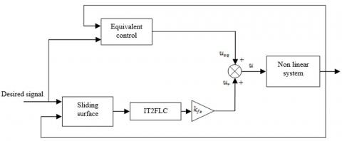
The control algorithms based on sliding mode techniques suffers from a main disadvantage that is chattering effect, which is the high frequency oscillation of the controller output. To overcome this problem and in order to reduce the chattering phenomenon, an interval type-2 fuzzy system is used to approximate the hitting control term. The configuration of the proposed type-2 fuzzy sliding mode control scheme is shown in Figure 4; it contains an equivalent control part and single input single output interval type-2 fuzzy logic.
Figure 4. Block diagram of the IT2FSMC
The equivalent control $u_{e q}$, is calculated in such a way as to have $\dot{s}=0 .$ Then the discontinuous control is computed by:
$u_{r}=k_{f s} u_{f s} \quad u_{f s}=I T 2 F L C(s)$ (26/27)
where:
$k_{f s}$ is the normalization factor of the output variable, and $u_{f s}$ is the output of the IT2FLC, which is obtained by the normalized $s$.
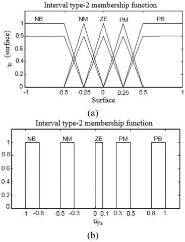
The fuzzy type- 2 membership functions of the input sliding surface $(s),$ and the output discontinuous control $\left(u_{f s}\right)$ sets =are presented by Figure 5.
Figure 5. Membership functions of input s and output $u_{f s}$
In order to attenuate the chattering effect and handle the uncertainty of the six rotors helicopter, a type- 2 fuzzy controller has been used with single input and single output for each subsystem. Then, the input of the controller is the sliding surface and the output is the discontinuous control $u_{f s} .$ All the membership functions of the fuzzy input variable are chosen to be triangular and trapezoidal for all upper and lower membership functions. The used labels of the fuzzy variable (surface) are: \{negative medium (NM), negative big (NB), zero (ZE), positive medium (NM), positive big (PB) $\}$.
The corrective control is decomposed into five levels represented by a set of linguistic variables: negative big (NB), negative medium (NM), zero (ZE), positive medium (PM) and positive big (PB). Table.1 presents the rules base which contains five rules:
Table 1. Fuzzy rules for type-2 FLCs
|
|
Rule 1 |
Rule 2 |
Rule 3 |
Rule 4 |
Rule 5 |
|
Surface |
PB |
PM |
ZE |
NM |
NB |
|
$u_{f s}$ |
NB |
NM |
ZE |
PM |
PB |
The membership functions of the input (sliding surface) and output $\left(u_{f s}\right)$ has been normalized in the interval [-1,1] therefore: $\left|u_{f s}\right| \leq 1$.
$u_{f s}$ given in equation (27) satisfies the following condition
$u_{f s}=-K^{+}|s|$ (28)
where: $K^{+}>0$ is positive constant determined by a fuzzy type-2 inference system.
Proof:
The discontinuous control laws are computed by type- 2 fuzzy logic inference using equations (19) and (20) and the iterative Karnik Mendel Algorithms presented in [26-30]. Where $\alpha_{i}=\left[\alpha_{\text {ilow }}, \alpha_{\text {iup }}\right]$ for $i=[1, \ldots, 5]$ are the membership interval of rules 1 to 5 presented in Table 1. Moreover, $u_{f s}$ can be further analyzed as the following six conditions given thereafter. Only one of six conditions will occur for any value of the sliding surface $s$ according to Figure 4.
Condition 1
Only rule 1 is activated $\left(s>0.5, \alpha_{1}=[0.8,1], \alpha_{j}=[0,0]\right)$ for $j=2,3,4,5$
$u_{f s}=I T 2 F L C(s)=\frac{-0.8-1}{2}=-0.9$ (29)
Condition 2
Rule 1 and 2 are activated $\left(0.25<s<0.5, \alpha_{1}=\right.$ $\left.\left[\alpha_{1 l o w}, \alpha_{1 u p}\right], \alpha_{2}=\left[\alpha_{2 l o w}, \alpha_{2 u p}\right], \alpha_{j}=[0,0]\right)$ for $j=3,4,5$
$0 \leq \alpha_{1 l o w}, \alpha_{2 l o w} \leq 0.8$ and $0 \leq \alpha_{1 u p}, \alpha_{2 u p} \leq 1$
$\begin{aligned} u_{f s}=\operatorname{IT} 2 F L C(s)=& \frac{1}{2}\left(\frac{-0.8 \alpha_{1 l o w}-0.3 \alpha_{2 u p}}{\alpha_{1 l o w}+\alpha_{2 u p}}\right.\\ &\left.+\frac{-\alpha_{1 u p}-0.5 \alpha_{2 l o w}}{\alpha_{1 u p}+\alpha_{2 l o w}}\right) \end{aligned}$ (30)
Condition 3
Rule 2 and 3 are activated $\left(0<s<0.25, \alpha_{2}=\left[\alpha_{2 l o w}, \alpha_{2 u p}\right], \alpha_{3}=\left[\alpha_{3 l o w}, \alpha_{3 u p}\right], \alpha_{j}=[0,0]\right)$ for $j=1,4,5$
$0 \leq \alpha_{2 l o w}, \alpha_{3 l o w} \leq 0.8$ and $0 \leq \alpha_{2 u p}, \alpha_{3 u p} \leq 1$
$\begin{aligned} u_{f s}=I T 2 F L C(s)=& \frac{1}{2}\left(\frac{-0.3 \alpha_{2 l o w}+0.1 \alpha_{3 u p}}{\alpha_{2 l o w}+\alpha_{3 u p}}\right.\\ &\left.+\frac{-0.5 \alpha_{2 u p}}{\alpha_{2 u p}+\alpha_{3 l o w}}\right) \end{aligned}$ (31)
Condition 4
Rule 3 and 4 are activated $\left(-0.25<s<0, \alpha_{3}=\right.$ $\left.\left[\alpha_{3 l o w}, \alpha_{3 u p}\right], \alpha_{4}=\left[\alpha_{4 l o w}, \alpha_{4 u p}\right], \alpha_{j}=[0,0]\right)$ for $j=1,2,5$
$0 \leq \alpha_{3 l o w}, \alpha_{4 l o w} \leq 0.8$ and $0 \leq \alpha_{3 u p}, \alpha_{4 u p} \leq 1$
$\begin{aligned} u_{f s}=\operatorname{IT} 2 F L C(s)=& \frac{1}{2}\left(\frac{0.1 \alpha_{3 l o w}+0.5 \alpha_{4 u p}}{\alpha_{3 l o w}+\alpha_{4 u p}}\right.\\ &\left.+\frac{0.3 \alpha_{4 l o w}}{\alpha_{3 u p}+\alpha_{4 l o w}}\right) \end{aligned}$ (32)
Condition 5
Rule 4 and 5 are activated $\left(-0.5<s<-0.25, \alpha_{4}=\right.$ $\left.\left[\alpha_{4 l o w}, \alpha_{4 u p}\right], \alpha_{5}=\left[\alpha_{5 l o w}, \alpha_{5 u p}\right], \alpha_{j}=[0,0]\right)$ for $j=1,2,3$
$0 \leq \alpha_{4 l o w}, \alpha_{5 l o w} \leq 0.8$ and $0 \leq \alpha_{4 u p}, \alpha_{5 u p} \leq 1$
$\begin{aligned} u_{f s}=\operatorname{IT} 2 F L C(s)=& \frac{1}{2}\left(\frac{0.5 \alpha_{4 l o w}+\alpha_{5 u p}}{\alpha_{4 l o w}+\alpha_{5 u p}}\right.\\ &\left.+\frac{0.3 \alpha_{4 u p}+0.8 \alpha_{5 l o w}}{\alpha_{4 u p}+\alpha_{5 l o w}}\right) \end{aligned}$ (33)
Condition 6
Only rule 5 is activated $\left(s<-0.5, \alpha_{5}=[0.8,1], \alpha_{j}=\right.$ [0,0]) for $j=1,2,3,4$
$u_{f s}=I T 2 F L C(s)=\frac{1+0.8}{2}=0.9$ (34)
According to six possible conditions shown in (29)-(34) we conclude
$u_{f s}=I T 2 F L C(s)=-K^{+}|s|$ (35)
with:
$K^{+}=\left\{\begin{array}{l}0.9 \,\,\,\,\,\,\,\,\,\,\,\,\,\,\,\,\,\,\,\,\,\,\,\,\,\,\,\,\,\,\,\,\,\,\,\,\,\,\,\,\,\,\,\,\,\,\,\,\,\,\,\,\,\,\,\,\,\,\,\,\,\,\,\,\,\,\,\,\,\,\,\,{if\,\,s>}0.5\,and\,s<-0.5 \\ \left|\frac{1}{2}\left(\frac{-0.8 \alpha_{1 l o w}-0.3 \alpha_{2 u p}}{\alpha_{1 l o w}+\alpha_{2 u p}}+\frac{-\alpha_{1 u p}-0.5 \alpha_{2 l o w}}{\alpha_{1 u p}+\alpha_{2 l o w}}\right)\right| \text { if } 0.25<s<0.5 \\ \left|\frac{1}{2}\left(\frac{-0.3 \alpha_{2 l o w}+0.1 \alpha_{3 u p}}{\alpha_{2 l o w}+\alpha_{3 u p}}+\frac{-0.5 \alpha_{2 u p}}{\alpha_{2 u p}+\alpha_{3 l o w}}\right)\right| \quad \text { if } 0<s<0.25 \\ \left|\frac{1}{2}\left(\frac{0.1 \alpha_{3 l o w}+0.5 \alpha_{4 u p}}{\alpha_{3 l o w}+\alpha_{4 u p}}+\frac{0.3 \alpha_{4 l o w}}{\alpha_{3 u p}+\alpha_{4 l o w}}\right)\right| \quad \text { if }-025<s<0 \\ \left|\frac{1}{2}\left(\frac{0.5 \alpha_{4 l o w}+\alpha_{5 u p}}{\alpha_{4 l o w}+\alpha_{5 u p}}+\frac{0.3 \alpha_{4 u p}+0.8 \alpha_{5 l o w}}{\alpha_{4 u p}+\alpha_{5 l o w}}\right)\right| \quad \text { if }-05<s<-0.25\end{array}\right.$ (36)
In Figure 4 the control law is computed by:
$u=u_{e q}+u_{r}=u_{e q}+k_{f s} u_{f s}$ (37)
Then sliding condition can be rewritten as follow:
$s \dot{\mathrm{s}}=-k_{f s} K^{+}|s|<0$ (38)
Or
$\dot{s}=-k_{f s} T 2 F L C(s)$ (39)
To obtain the type-2 fuzzy sliding mode control of a doubly-fed induction machine, the surfaces are chosen according to the error between the reference input signal and the measured signals as follows:
4.4 Speed control
For $n=1,$ the speed control manifold can be obtained from equation (22) as follow:
$S(\Omega)=\Omega_{r e f}-\Omega$ (40)
The derivative of the surface is:
$\dot{S}(\Omega)=\dot{\Omega}_{r e f}-\dot{\Omega}$ (41)
Substituting the expression of $\dot{\Omega}$ equation (11) in equation (41), we obtain:
$\dot{S}(\Omega)=\dot{\Omega}_{r e f}+\frac{1}{J}\left(\frac{p \cdot M}{L_{s}} \varphi_{s d} I_{r q}+f \Omega+C_{r}\right)$ (42)
To find the expression of the control law equates equation (42) by equation (39), we obtain:
$\begin{aligned} \dot{\Omega}_{r e f}+\frac{1}{J}\left(\frac{p \cdot M}{L_{S}} \varphi_{s d} I_{r q}+f \Omega+C_{r}\right) \\ &=-k_{f s \Omega} T 2 F L C(s(\Omega)) \end{aligned}$ (43)
So:
$I_{r q}=-\frac{J L_{s}}{p M \varphi_{s d}}\left(\dot{\Omega}_{r e f}+\frac{f}{J} \Omega+\frac{C_{r}}{J}\right)-\frac{J L_{s}}{p M \varphi_{s d}} k_{f s \Omega} T 2 F L C(s(\Omega))$ (44)
We take: $I_{r q}^{r e f}=I_{r q}^{e q}+I_{r q}^{n},$ with:
$\left\{\begin{array}{l}I_{r q}^{e q}=-\frac{J L_{S}}{p M \varphi_{s d}}\left(\dot{\Omega}_{r e f}+\frac{f}{J} \Omega+\frac{C_{r}}{J}\right) \\ I_{r q}^{n}=-\frac{J L_{S}}{p M \varphi_{s d}} k_{f s \Omega} T 2 F L C(s(\Omega))\end{array}\right.$ (45)
To check the stability condition of the system, the constant $k_{f s \Omega}>0$.
4.5 Stator flux oriented control
In the proposed control, the manifold equation can be obtained by:
$S\left(\varphi_{s d}\right)=\varphi_{s d}^{r e f}-\varphi_{s d}$
$\dot{S}\left(\varphi_{s d}\right)=\dot{\varphi}_{s d}^{r e f}-\dot{\varphi}_{s d}$ (46)
Substituting the expression of $\dot{\varphi}_{s d}$ equation (10) in equation (46), we obtain:
$\dot{S}\left(\varphi_{s d}\right)=\dot{\varphi}_{s d}^{r e f}-\left(V_{s d}+\frac{M}{T_{s}} I_{r d}-\frac{1}{T_{s}} \varphi_{s d}\right)$ (47)
To find the expression of the control law equates equation (47) by equation (39), we obtain:
$\begin{aligned} \dot{\varphi}_{s d}^{r e f}-\left(V_{s d}+\frac{M}{T_{s}}\right.&\left.I_{r d}-\frac{1}{T_{s}} \varphi_{s d}\right) \\ &=-k_{f s \varphi_{s d}} T 2 F L C\left(s\left(\varphi_{s d}\right)\right) \end{aligned}$ (48)
So:
$\begin{aligned} I_{r d}=\frac{T_{S}}{M}\left(\dot{\varphi}_{s d}^{r e f}-\right.&\left.V_{s d}+\frac{1}{T_{S}} \varphi_{s d}\right) \\ &+\frac{T_{S}}{M} k_{f s \varphi_{s d}} T 2 F L C\left(s\left(\varphi_{s d}\right)\right) \end{aligned}$ (49)
The control current $I_{r d}$ is defined by: $I_{r d}^{r e f}=I_{r d}^{e q}+I_{r d}^{n},$ with:
$\left\{\begin{array}{l}I_{r d}^{e q}=\frac{T_{s}}{M}\left(\dot{\varphi}_{s d}^{r e f}-V_{s d}+\frac{1}{T_{s}} \varphi_{s d}\right) \\ I_{r d}^{n}=\frac{T_{s}}{M} k_{f s \varphi_{s d}} T 2 F L C\left(s\left(\varphi_{s d}\right)\right)\end{array}\right.$ (50)
To check the stability condition of the system, the constant $k_{f s \varphi_{s d}}>0$.
4.6 Rotor direct current control
The expression of the control surface of the current $I_{r d}$ is given by:
$S\left(I_{r d}\right)=I_{r d}^{r e f}-I_{r d}$ (51)
The derivative of the surface is:
$\dot{S}\left(I_{r d}\right)=\dot{I}_{r d}^{r e f}-\dot{I}_{r d}$ (52)
Substituting the expression of the current $\dot{I}_{r d}$ equation (10), we obtain:
$\dot{S}\left(I_{r d}\right)=\dot{I}_{r d}^{r e f}-\left(-\delta I_{r d}+\left(\omega_{s}-\omega\right) I_{r q}+\alpha \varphi_{s d}\right.$
$\left.-\frac{M}{\sigma L_{s} L_{r}} V_{s d}+\frac{1}{\sigma L_{r}} V_{r d}\right)$ (53)
Equates equation (53) by equation (39), we obtain:
$\begin{aligned} \dot{I}_{r d}^{r e f}-\left(-\delta I_{r d}+\left(\omega_{S}-\omega\right) I_{r q}+\alpha \varphi_{s d}-\frac{M}{\sigma L_{S} L_{r}} V_{s d}\right.\\+\frac{1}{\sigma L_{r}} V_{r d} &=-k_{f s I_{r d}} T 2 F L C\left(s\left(I_{r d}\right)\right) \end{aligned}$ (54)
So:
$V_{r d}=\left(i_{r d}^{r e f}+\delta I_{r d}+\frac{M}{\sigma L_{s} L_{r}} V_{s d}-\alpha \varphi_{s d}-\left(\omega_{s}-\omega\right) I_{r q}\right) \sigma L_{r}+\sigma L_{r} k_{f s I_{I d}} T 2 F L C\left(s\left(I_{r d}\right)\right)$ (55)
The equation (55) can be rewritten by: $V_{r d}^{r e f}=V_{r d}^{e q}+V_{r d}^{n}$, with:
$\left\{\begin{array}{l}\mathrm{V}_{r d}^{e q}=\left(I_{r d}^{r e f}+\delta I_{r d}+\frac{M}{\sigma L_{S} L_{r}} V_{s d}-\alpha \varphi_{s d}-\left(\omega_{s}-\omega\right) I_{r q}\right) \sigma L_{r} \\ V_{r d}^{n}=\sigma L_{r} k_{f s I_{r d}} T 2 F L C\left(s\left(I_{r d}\right)\right)\end{array}\right.$ (56)
To check the stability condition of the system, the constant $k_{f s I_{r d}}>0$.
4.7 Rotor quadrature current control
The expression of the control surface and the derivative of the current $I_{r q}$ defined by:
$\left\{\begin{array}{l}S\left(I_{r q}\right)=I_{r q}^{r e f}-I_{r q} \\ \dot{S}\left(I_{r q}\right)=\dot{I}_{r a}^{r e f}-\dot{I}_{r q}\end{array}\right.$ (57)
We replace the expression of the current $\dot{I}_{r q}$ (equation 10 ), we obtain:
$\dot{S}\left(I_{r q}\right)=\dot{I}_{r q}^{r e f}-\left(-\left(\omega_{s}-\omega\right) I_{r d}-\delta I_{r q}+\beta \omega \varphi_{s d}\right.$
$\left.-\frac{M}{\sigma L_{s} L_{r}} V_{s q}+\frac{1}{\sigma L_{r}} V_{r q}\right)$ (58)
Equates equation (58) by equation (39), we obtain:
$\dot{I}_{r q}^{r e f}-\left(-\left(\omega_{s}-\omega\right) I_{r d}-\delta I_{r q}+\beta \omega \varphi_{s d}-\frac{M}{\sigma L_{s} L_{r}} V_{s q}+\frac{1}{\sigma L_{r}} V_{r q}\right)=-k_{f s I_{r q}} T 2 F L C\left(s\left(I_{r q}\right)\right)$ (59)
So:
$\begin{aligned} V_{r q}=\left(i_{r q}^{r e f}+\left(\omega_{s}-\omega\right) I_{r d}+\delta I_{r q}-\beta \omega \varphi_{s d}\right.\\ &\left.+\frac{M}{\sigma L_{s} L_{r}} V_{s q}\right) \sigma L_{r} \\ &+\sigma L_{r} k_{f s I_{r q}} T 2 F L C\left(s\left(I_{r q}\right)\right) \end{aligned}$ (60)
The equation (60) can be rewritten by: $V_{r q}^{r e f}=V_{r q}^{e q}+V_{r q}^{n}$
with:
$\left\{\begin{array}{l}\mathrm{V}_{r q}^{e q}=\left(i_{r q}^{r e f}+\left(\omega_{s}-\omega\right) I_{r d}+\delta I_{r q}-\beta \omega \varphi_{s d}+\frac{M}{\sigma L_{s} L_{r}} V_{s q}\right) \sigma L_{r} \\ V_{r q}^{n}=\sigma L_{r} k_{f s I_{r q}} T 2 F L C\left(s\left(I_{r q}\right)\right)\end{array}\right.$ (61)
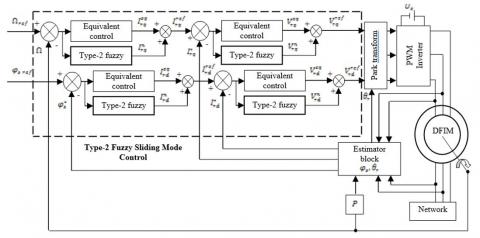
Figure 6. Block diagram of the Type-2 Fuzzy Sliding Mode control of the DFIM
To check the stability condition of the system, the constant $k_{f s I_{r q}}>0$.
The structure of type-2 fuzzy sliding mode control of a doubly-fed induction machine is shown in the figure 6. It is similar to the structure of a Sliding Mode control; the control kept the part of the equivalent control and will change the part of the switching by a type-2 fuzzy controller.
The objective of this step is to control the DFIM by the hybrid type-2 fuzzy sliding mode control of which the stator of the machine is powered directly by the three-phase network [220 / 380V, 50Hz] and the rotor is supplied with voltage through a PWM inverter. The parameters of the DFIM used in this work are given in the appendix.
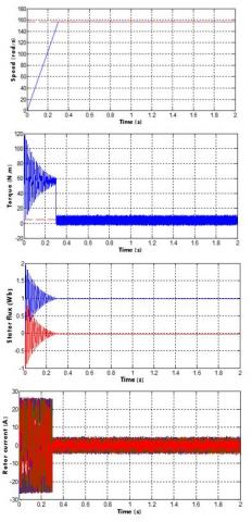
The simulation results are grouped together in Figure $7 .$ The speed of the machine has a first order response of end value $157(\mathrm{rad} / \mathrm{s}) .$ Between instants $t=0.6 s$ and $t=1.6 s$ is applied a charge of value $C_{r}=10 \mathrm{N} . \mathrm{m}$. We find that the load variation does not influence the speed and flux quantities. The principle of vector control is verified by the decoupling between flux and torque.
Figure 7. Simulation results of the DFIM controlled by type-2 fuzzy sliding mode control
In the second test, is applied a load of value $C_{r}=$ $5 N . m$ between instants $t=0.6 s$ and $t=1.6 s$ a variation on the rotor resistance at $(+100 \%) .$ We do not see that the variation of the rotor resistance does not affect the speed and flux quantities. The principle of vector control is always verified.
Figure 8. Type-2 fuzzy sliding mode control of the DFIM with rotor resistance variation
In the present study, an integral squared error (ISE), integral absolute error (IAE) and integral time-weighted absolute error (ITAE) are utilized to judge the performance of the controllers. ISE, IAE and ITAE criterion is widely adopted to evaluate the dynamic performance of the control system. The index ISE, IAE and ITAE is expressed as follows:
$\mathrm{ISE}=\int_{0}^{T} e^{2}(t) d t$ (62)
$\mathrm{IAE}=\int_{0}^{T}|e(t)| d t$ (63)
$\mathrm{ITAE}=\int_{0}^{T} t|e(t)| d t$ (64)
For quantitative comparison between two methods, ISE, IAE and ITAE are used as the criterion. Table.3 shows the ISE, IAE and ITAE values of the simulation results using the vector control proposed in [31], sliding mode control proposed in [32] and the proposed Controller. From the comparison, it can be seen that the performance is improved when using the proposed controller as compared to the anther methods. Actually these performances index are obtained at the end of the simulation time (T=2 sec) with a sampling period h=10-4.
Table 2. ISE, IAE and ITAE performance indexes
|
Controllers Index |
Direct field-oriented control proposed in [31] |
Sliding mode control proposed in [32] |
Proposed controller |
|
|
ISE |
Speed |
16600 |
13400 |
10300 |
|
flux |
0.134 |
0.122 |
0.089 |
|
|
IAE |
Speed |
84.514 |
74.521 |
50.069 |
|
flux |
0.305 |
0.202 |
0.056 |
|
|
ITAE |
Speed |
15.306 |
11.203 |
4.207 |
|
flux |
0.1532 |
0.105 |
0.0156 |
|
It can be concluded that the system performances are better, when using the proposed control as compared to the control methods proposed in [31, 32].
This paper presents hybrid type 2 fuzzy sliding mode control of the doubly fed induction machine and performance evaluations. After presenting a Mathematical modeling of DFIM, we applied the orientation of stator flux to have the decoupling between the flux and the current for simplified the model of DFIM.
Hybrid type 2 fuzzy sliding mode control use the equivalent control by sliding mode and the switching by type 2 fuzzy controller. Simulations were investigated with this type controller and they showed very interesting performances in terms of reference tracking, sensitivity to perturbation and robustness under parameter variation.
In the futures works we propose another controls techniques for example the adaptive interval type 2 fuzzy controller of the DFIM, fusion of neural networks with fuzzy techniques and high-order sliding mode control.
Parameters of the DFIM [5]:
|
Parameters |
Value |
|
Nominal power |
$P_{n}=4 K W$ |
|
Stator voltage |
$U_{s n}=380 \mathrm{V}$ |
|
Rotor voltage |
$U_{r n}=220 \mathrm{V}$ |
|
Nominal current |
$I_{n}=15 / 8.6 A$ |
|
Nominal mechanical speed |
$\Omega_{n}=1440 \mathrm{rpm}$ |
|
Nominal stator and rotor frequencies |
$\omega_{s n}=50 H z$ |
|
Pole pair number |
P=2 |
|
Stator resistance |
$R_{s}=1.2 \Omega$ |
|
Rotor resistance |
$R_{r}=1.8 \Omega$ |
|
Stator self inductance |
$L_{s}=0.1554 H$ |
|
Rotor self inductance |
$L_{r}=0.1568 H$ |
|
Mutual inductance |
$M=0.15 H$ |
|
Moment of inertia |
$J=0.2 \mathrm{Kg} \cdot \mathrm{m}^{2}$ |
|
Friction coefficient |
$f=0.001 I S$ |
Nomenclature:
|
s, r |
Stator and rotor subscripts |
|
d, q |
Direct and quadrate Park subscripts |
|
V, I, φ |
Voltage/ Current/ Flux variables |
|
$R_{s}, R_{r}$ |
Stator, rotor resistance |
|
$L_{s}, L_{r}$ |
Stator, rotor inductance |
|
$T_{s}, T_{r}$ |
Statoric and rotoric time-constant |
|
$\theta_{s}, \theta_{r}$ |
Statoric and rotoric flux position |
|
σ |
Leakage factor |
|
$\omega_{s}$ |
Electrical stator frequency |
|
ω |
Mechanical rotor frequency |
|
Ω |
Mechanical speed |
|
$C_{e m}$ |
Electromagnetic torque |
|
$C_r$ |
External load torque |
|
PWM |
Pulse width modulation |
|
T2FLC |
Type 2 fuzzy logic controllers |
|
DFIM |
doubly fed induction machine |
[1] Vidal, P.E. (2004). Commande non-linéaire d'une machine asynchrone à double Alimentation. Doct. Thesis, Dept. of Elect. Eng., National Polytechnic Institute of Toulouse, France.
[2] Salloum, G. (2007). Contribution à la commande robuste de la machine asynchrone à double alimentation. Doct. Thesis, Dept. of Elect. Eng, National Polytechnic Institute of Toulouse, France.
[3] Vicatos, M.S., Tegopoulos, J.A. (2003). A Doubly-fed induction machine differential drive model for automobiles. IEEE Trans. Ene. Conv., 18(2): 225-230. https://doi.org/10.1109/TEC.2003.811732
[4] Bekakra, Y., Ben attous, D. (2010). Speed and flux control for DFOC of doubly fed induction machine using sliding mode controller. Acta Electrotechnica et Informatica, 10(4): 75-81.
[5] Rouabhi, R. (2016). Contrôle des puissances générées par un système éolien à vitesse variable basé sur une machine asynchrone double alimentée. Doct. Thesis, Dept. of Elect, university of Batna, Algeria.
[6] Blaschke, E. (1972). Principe of field orientation as applied to the new transvector closed loop control system for rotating field machine. Siemens Review, 34: 217-220.
[7] Chaari, M., Soltani, M., Gossa, M. (2007). Comparative study between the conventional regulators and fuzzy logic controller: application on the induction machine. International Journal of Sciences and Techniques of Automatic control & computer engineering IJ-STA, 1(2): 196-212.
[8] Nasri, A., Hazzab, A., Bousserhane, I.K., Hadjiri, S., Sicard, P. (2008). Two wheel speed robust sliding mode control for electrical vehicle drive. Serbian Journal of Electrical Engineering, 5(2): 199-216. https://doi.org/10.2298/SJEE0802199A
[9] Shim, H.S., Kim, J.H., Koh, K. (1995). Variable structure control of non holonomic mobile robots. IEEE conf. Robot. Automat, 1694-1699. https://doi.org/10.1109/ROBOT.1995.525517
[10] Yang, J.M., Choi, I.H., Kim, J.H. (1999). Sliding mode motion control of non holonomic mobile robots. IEEE control system, 19(19): 15-23. https://doi.org/10.1109/37.753931
[11] Ishigame, A., Furukawa, T. (1993). Sliding mode controller design based on fuzzy inference for nonlinear systems. IEEE transactions on industrial Electronics, 40(1). https://doi.org/10.1109/IECON.1991.239018
[12] Boucheta, A., Bousserhane, I.K., Hazzab, A., Mazari, B., Fellah, M.K. (2009). Fuzzy-Sliding Mode Controller for Linear Induction Motor Control. Rev. Roum. Sci. Techn. – Électrotechn. Et Énerg., 54(4): 405-414.
[13] Bouguerra, A., Zeghlache, S., Loukal, K., Saigaa, D. (2016). Fault Tolerant Fuzzy Sliding Mode Controller of Brushless DC Motor (BLDC MOTOR). the Mediterranean Journal of Measurement and Control, 12(2): 585-597.
[14] Ardjoun, S.A., Abid, M., Aissaoui, A.G., Tahour, A. (2012). A Robust Sliding Mode Control Applied to The Double Fed Induction Machine. IU-JEEE, 12(1): 1445-1451.
[15] Boyette, A. (2006). Contrôle-commande d’un générateur asynchrone à double alimentation avec système de stockage pour la production eolienne. Doct. Thesis, Dept. of Elect. Eng, University Henri Poincaré, Nancy I, France. https://doi.org/10.2514/1.21882
[16] Berrabah, F., Chebabhi, A., Zeghlache, S. (2017). Direct torque control of induction motor fed by three-level inverter using fuzzy logic. AMSE Journals, Series Advances C., 72: 248-265.
[17] Belhamdi, S., Goléa, A. (2017). Direct field-oriented control using fuzzy logic type-2 for induction motor with broken rotor bars. AMSE Journals, Series Advances C., 72: 203-212.
[18] Mendel, J.M., John, R.I., Liu, F. (2006). Interval type-2 fuzzy logic systems made simple. IEEE Transactions on Fuzzy Systems, 14(6): 808-818. https://doi.org/10.1109/TFUZZ.2006.879986
[19] Mendel, J. (2001). Uncertain rule-based fuzzy logic systems: introduction and new directions. Prentice-Hall.
[20] Hagras, H.A. (2004). A hierarchical type-2 fuzzy logic control architecture for autonomous mobile robots. IEEE Trans. Fuzzy Syst, 12(4): 524-539. https://doi.org/10.1109/TFUZZ.2004.832538
[21] Liang, Q., Mendel, J.M. (2000). Interval type-2 fuzzy logic systems: theory and design. IEEE Transactions on Fuzzy Systems, 8(5): 535-550. https://doi.org/10.1109/91.873577
[22] Ezziani, N. (2010). Commande adaptative floue backstepping d’une machine asynchrone avec et sans capteur mecanique. Doct. Thesis in Computer Engineering, automatic and signal processing, Reims University, France.
[23] Loukal, K., Benalia, L. (2015). Type-2 Fuzzy Logic Control of a Doubly-Fed Induction Machine (DFIM). IAES International Journal of Artificial Intelligence (IJ-AI), 4(4): 139-152. https://doi.org/10.11591/ijai.v4.i4.pp139-152
[24] Slotine, W., Li, J.J.E. (1998). Applied nonlinear control. Prence Hall, USA.
[25] Lopez, P., Nouri, A.S. (2006). Théorie Elémentaire Et Pratique de La Commande Par Les Régimes Glissants. Springer. https://doi.org/10.1007/3-540-34480-2
[26] Castillo, O., Melin, P. (2012). A review on the design and optimization of interval type-2 fuzzy controllers. Applied Soft Computing, 12: 1267-1278. https://doi.org/10.1016/j.asoc.2011.12.010
[27] Juan, R., Castillo, O., Melin, P., Díaz, A.R. (2009). A hybrid learning algorithm for a class of interval type-2 fuzzy neural networks. Information Sciences, 179: 2175-2193. https://doi.org/10.1016/j.ins.2008.10.016
[28] Martínez, R., Castillo, O., Aguilar, L. (2009). Optimization of interval type-2 fuzzy logic controllers for a perturbed autonomous wheeled mobile robot using genetic algorithms. Information Sciences, 179: 2158-2174. https://doi.org/10.1016/j.ins.2008.12.028
[29] Wu, D., Tan, W. (2006). A simplified type-2 fuzzy logic controller for real-time control. ISA Transactions, 45: 503-510. https://doi.org/10.1016/S0019-0578(07)60228-6
[30] Castillo, O., Marroquín, M., Melin, P., Valdez, F., Soria, J. (2012). Comparative study of bio-inspired algorithms applied to the optimization of type-1 and type-2 fuzzy controllers for an autonomous mobile robot. Information Sciences, 192: 19-38. https://doi.org/10.1016/j.ins.2010.02.022
[31] Rouabhi, R., Abdessemed, R., Chouder, A., Djerioui, A. (2015). Hybrid Backstepping control of a doubly fed wind energy induction generator. The Mediterranean Journal of Measurement and Control, 11(1): 367-376.
[32] Belounis, O., Labar, H. (2017). Fuzzy Sliding Mode Controller of DFIG for Wind Energy Conversion. International Journal of Intelligent Engineering and Systems, 10(2): 163-172, 2017. https://doi.org/10.22266/ijies2017.0430.18