Soumia Ourrad*![]() | Youcef Houmadi | Sidi Mohammed Aissa Mamoune | Abdelkader Ziadi
| Youcef Houmadi | Sidi Mohammed Aissa Mamoune | Abdelkader Ziadi![]()
© 2023 IIETA. This article is published by IIETA and is licensed under the CC BY 4.0 license (http://creativecommons.org/licenses/by/4.0/).
OPEN ACCESS
Over the past ten years, Cr-Mo is used for the manufacture of hydro treating reactors, in order to meet the demand of the refining industry, steelmakers have had to develop Cr-Mo steel, which until then was widely used for the manufacture of devices operating at high temperatures under hydrogen pressure The purpose of this work is to study the susceptibility of steel 42CrMo4 (AISI4041) to hydrogen this steel is a martensitic, that is widely use especially in the hydrogen storage industry, this one is tempered at different temperatures (500, 550, 600, 650 and 700℃), the application of artificial neural networks is proposed to predict the optimum tempering temperature to have a minimal quantity of hydrogen by analyzing the hydrogen concentration parameter that escapes through the desorption phenomenon through time at room temperature the Mathematical model proposed by the neural network method has proved this and this has been validated once more by comparing it with a global statistical study following a coupling between the variables “time / concentration”, “Tempering Temperature / concentration”. In addition, the data used in the model were taken from real experimental data and are arranged in a format of two input parameters: time and tempering temperature, and output parameter is hydrogen concentration. The model was arbitrated using Mean Absolute Error (MAE) and average quadratic error (MSE) and correlation coefficient and model performance values found as 0.0686 and 0.0071, 98.87%, 0.0071 for the training part and 0.0916 and 0.0112, 99.10%, 0.0112 for the test. Finally, the major conclusions of this research show that ANN as powerful computational techniques in modeling of nonlinear systems, can be reliably used in the prediction and correlation to obtain tempering temperature to get lower hydrogen concentration lesser.
hydrogen concentration, neural networks, prediction, 42CrMo4 steel
The evolution of techniques and processes, research for the highest efficiencies, the reductions of cost make that materials can be brought to work in more hard conditions for the hydrogen in high pressure raised brought up 70 MPa where from the steel development of high strength. Significant changes in steels, in the techniques of development and transformation, in their implementation, always involve new studies [1]. Increasingly, users of hydrogen-sensitive metal parts, reactors or structures wish to have reliable techniques or models for predicting, monitoring and controlling the evolution of hydrogen to avoid damage during service [1].
The situations that can lead to hydrogen embrittlement phenomena are numerous, such as the penetration of this gas during production or during conversion and hydrogen processing operations resulting from corrosion reactions (aqueous environments).
Hydrogen embrittlement can manifest itself in various forms depending on the state of the material of its microstructural composition and the stress conditions as well as surrounding environment. 42CrMo4 steel is an alloy steel with a medium carbon content that is usually used in quenching and tempering when it requires an optimal combination of strength and toughness. In addition, it offers high resistance to fatigue and wear, making it an excellent candidate for the manufacture of fabrication, for example, containers for storing and transporting gaseous hydrogen at high pressures. However, it is known that high-strength steel, as is the case for 42CrMo4 steel, is susceptible to hydrogen embrittlement and that in addition, the susceptibility is proportional to the increase in the mechanical strength of steel [2-4]. The motivation of this research is to define the optimum tempering temperature (heat treatment) which allows having a material sufficiently resistant to hydrogen embrittlement and resists longer.
The human brain contains about 100 billion neurons. These neurons allow us to read a text while maintaining a regular breathing allowing oxygenating our blood, by activating our heart which ensures an efficient circulation of this blood to feed our cells, etc. It is generally believed that their different neuronal functions, including that of memory, are stored in the connections (synapses) between neurons. This kind of theory that has inspired most architectures of artificial neural networks (so-called "formal"). Learning involves establishing new connections, or modifying existing connections. The first studies for the resolution of this problem were establish in the laboratory AT&T by using neurons network named LeTNet which uses a representation by pixel [5]. In 1992, Knerr proposed a very different approach which consists in realizing an image preprocessing in order to extract discriminating characteristics which allow to use one to classify relatively simple [5, 6]. Applications are numerous such as the non-destructive testing, prediction of glass liquidus temperature, Kim and Sanders Jr [7] established a model on the basis on neural networks, for prediction of this temperature with a rather remarkable reliability with specific establishment of the bases of data for every glass they lied that: procedure has three advantages: (I) it is known that with more data, there is less over fitting in the ANN; (II) this procedure enables a voting process, which is expect to increase the identification accuracy; (III) the ANN can recognize a shifted spectrum caused by the calibration drift or a temperature change, Excitement of experimental system by combining defect and by one collects of the RMS (gap quadrature with regard an average, g) as relevant characteristic value for the state system. The obtained subset of characteristics so is to inject it in the neuron network [5]; in 1993, Zielinska applied to robot control systems especially to sensor data processing and solution of cinematic and dynamics problem; another application in electronic domain: Sensor less control of dc drive and an artificial neural network model for road accident prediction: A case study of a developing country [8]. Direct application in mechanical engineering is prediction of vibrations led by defects tricks [9].
Artificial neural networks helped to define that the right tempering temperature is 650℃ and 700℃ these temperatures allowed to reduce hydrogen concentration which was initially equal to 1.84 ppm which was reduced to 0.692 ppm.
To achieve this goal the manuscript has been subdivided into several titles, an overview of the history of artificial neural networks application and these uses in engineering field in the introductory part, The second title given to the soft computing techniques is the reasoning of this method then methodology which presents collection and processing of data then a comparative study was made between a statistical analysis and the said method analysis by the artificial neural networks, which first includes preparing training, validation and test data sets and in the second place preprocessing data for artificial neural network then presentation of results and their discussion and at the end a conclusion summarizing all results obtained.
According to Zadeh [10] soft computing is a collection of methodologies is which aim at exploiting tolerance in the imprecision and the uncertainty to reach a good robustness of the low-cost solution. His main constituents are the fuzzy logic, neuro-computing, and the probability reasoning [11]. This study involves the application of neurons network of the initials of which are ANN for the modelling of the concentration of the hydrogen within the metal due to its weakening effect. ANN context will be briefly explained in the following parts.
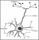
The neurons network is a functional concept of the biological neuronal structure of the central nervous system it consists of a large number of simple units of treatment known as neurons which are connected some to the others to train a network of thick connection [12]. The connections have weights associated with them called synaptiques weights. Every signal travel along a connection is multiplied by the weight of connection. The weights could be renewed for all the new data. Having realized a current database, the system training is easily updated with the data, which will be obtained later [13]. This method imitates the behavior of the human brain [14]. Mc Culloch et al. introduced the concept of neural networks; they developed the first model of neuronal network for the first time and developed a model cellular as in the Figure 1 [15, 16]. Mujrkhi constructed a model with two hidden layers feed-forward type of ANN for prediction the mechanical behavior [17].
Figure 1. Example of biologic neuron [18]
Collection and preparation of data of samples constitute the first stage of ANN conception model a total of 48 samples were carried out as a result each sample was tempered to a given temperature from 550, 600, 650, 700℃ so the concentration of each sample was measured in a moment "t" so Table 1 was obtained and the latter contains all data which are concentration (ppm), temperature (degree Celsus) and duration (hour) these values represents hydrogen release from the steel of which the chemical composition is express in percentage are C(0.42), Mn(0.62), Si(0.18), Cr(0.98), Mo(0.22), Cu(0.02), V(0.01). And this steel is subject to heat treatment named tempering at different temperatures from 500°C to 700℃ with a step of 50℃ during a rough duration of 700 hours for the steel 42CrMo4 (AISI4140) and that makes a set of 48 samples analyses. A descriptive statistical analysis was realized to obtain the information and the effects of the parameters considered in the present study. To allow the descriptive statistical analysis spread to the limits of the domain of modelling, it is guaranteed that the extreme value (values minimum and maximum) of every component of the total database is included in the descriptive database, the maximal value, the minimal value, the average gap, and every constituent, the Table 2 shows the statistical parameters of the data used for the statistical analysis.
Table 1. Database used for modeling where “t” is time and” Ch2 “is concentration and “T” is tempering temperature [4]
|
t (h) |
Ch2 (ppm) |
T (°C) |
|
4,53871 |
1,84374 |
500 |
|
7,18093 |
1,78155 |
500 |
|
30,7488 |
1,78171 |
500 |
|
50,3351 |
1,92324 |
500 |
|
52,9816 |
1,84974 |
500 |
|
118,489 |
1,74274 |
500 |
|
143,415 |
1,61284 |
500 |
|
215,473 |
1,49459 |
500 |
|
287,497 |
1,46682 |
500 |
|
385,63 |
1,64283 |
500 |
|
479,91 |
1,62088 |
500 |
|
625,343 |
1,36175 |
500 |
|
0,001 |
1,7205 |
550 |
|
0,58 |
1,6 |
550 |
|
117,43 |
1,36 |
550 |
|
311,72 |
1,3 |
550 |
|
454,75 |
1,13 |
550 |
|
503,9 |
1,01 |
550 |
|
696,014 |
0,95 |
550 |
|
0,01 |
1,4139 |
600 |
|
1,3136 |
1,15748 |
600 |
|
2,14648 |
1,10469 |
600 |
|
24,7098 |
0,93093 |
600 |
|
48,2689 |
0,919285 |
600 |
|
118,915 |
0,842879 |
600 |
|
217,498 |
0,773619 |
600 |
|
286,404 |
0,704778 |
600 |
|
336,198 |
0,756859 |
600 |
|
386,776 |
0,692048 |
600 |
|
0,01 |
1,21029 |
650 |
|
0,965329 |
0,910553 |
650 |
|
6,24992 |
0,80879 |
650 |
|
28,6589 |
0,509204 |
650 |
|
52,3256 |
0,351015 |
650 |
|
119,239 |
0,277966 |
650 |
|
214,993 |
0,233398 |
650 |
|
287,096 |
0,30743 |
650 |
|
552,037 |
0,247092 |
650 |
|
0,45787105 |
1,2052991 |
700 |
|
8,163819 |
0,81037194 |
700 |
|
31,61596 |
0,5055904 |
700 |
|
54,25522 |
0,3587637 |
700 |
|
119,69149 |
0,27932772 |
700 |
|
219,18307 |
0,23349784 |
700 |
|
289,91522 |
0,30821297 |
700 |
|
456,626 |
0,28071257 |
700 |
|
554,3761 |
0,24617706 |
700 |
Table 2. Statistics of variables (t,Ch2,T)
|
Descriptive Statistics |
|||||
|
|
N |
Min |
Max |
Mean |
Std. Deviation |
|
t |
47 |
0,01000 |
6,96014E2 |
1,9912786E2 |
2,01414483E2 |
|
Ch2 |
48 |
0,23339 |
1,92324 |
0,9969438 |
0,55178585 |
|
T |
48 |
500 |
700 |
596,87 |
73,228 |
The purpose of statistical analysis is to identify trends. It allows for the identification of patterns in unstructured and semi-structured processed data to make the experience richer.
The statistical analysis can be decomposed into five stages:
•Describe the nature of the data to be analyzed.
•Explore the relation between the data and the corresponding population.
•Create a model to synthesize the relations between the data and the population.
•Prove (or refute) the validity of the model.
•Use predictive analytics to develop scenarios that guide future actions.
In this study, the yield (efficiency) gives the results to adapt a multiple linear model to describe the relationship between concentration Ch2 and two independent variables, which are time and temperature. The equation of the adapted model is
$C=5,1274-0,000876078 * t-0,00664211 * T$ (1)
The statistical parameter value obtained P is lower than 0,05 leads the existence of a good relation between variables with a reliable level estimated at 95,0%. The correlation coefficient of the model is equal to 84,8875% of the variability of the concentration as well as the coefficient of adjusted correlation, which is more suited to compare models with various numbers of the independent variables, is 84.2006% the dispersal of the given is illustrated on the Figure 2.
Therefore, the variables involved in the hydrogen release are considered correlated.
Figure 2. Variation of concentration according to temperature and time
Usually, the complete set containing all available data sets of system behavior is divided into three subsets, called training subsets, validation subsets, and test subsets. The training subset, consisting of 70% random samples from the complete database, will be essentially in the training process on the other hand, the validation subset, compound 1% of the complete data set, allows to verify if the network capacities for the generalizing solutions are for acceptable levels, so allowing the test subset compound 15% of the complete data set is used to estimate the performances of prediction model. The algorithm of Levenberg Marquardt carried out formation of network in order to adjust the weights and the effectiveness of the training, the weights are adjusted to make the outputs (predictive) close to the target outputs (measured in experiments) of the network. The sum of the modified weights and bias was modified then by tansigmoïde transfer function. In the same way, the output of the hidden layer was modified by a suitable weight and the sum of the output signal modified again by tansigmoïde transfer function. After the completion of the formation process, the validation of neurons network is carried out. The neurons network was tested to determine the performance of the ANN model to predict the performance parameters. It was assured that the extreme values (values minimum and maximum) of each component of all data are integrated in all training data, all validation data and test, maximum value, minimal value, average deviation, and standard deviation of each parameter. Moreover, a procedure of bivariate correlation calculates the taub-b of Kendall with the level of significance used. The correlations measure the relation between the variables or the orders of classification. A procedure of bivariate correlation computes the pairwise associations for the definite variables (time/concentration, /concentration temperature), with resulting from this stage, the estimate curve concentration of hydrogen as a function of variable dependent on other independent variables (parameters above) are established. The representations of scatter chart (Figure 3a and 3b) show the estimate curve compared to the parameters already quoted. The Curve Estimation procedure produces curve estimation regression statistics and produce related plots for five (05) different curve estimation models. A separate model was produced for each dependent variable. The estimation of the most suitable curve is when the relation between the dependent variable (concentration) and the independent variable (time, Temperature) is not necessary linear. The coefficient of correlation R is the most parameter which estimates the proportion of total variation of the series which is explained by model.
(a)
(b)
Figure 3. (a) variation of concentration according to time, (b) variation of concentration according to temperature
For various models: linear, logarithmic curve, quadratic, power and exponential, R² was calculate it is illustrated on Table 3 and Table 4.
The correlation coefficient R² is the most important parameter that estimates the proportion of total variation in the series explained by the model. For each model (linear, logarithmic, quadratic, power, exponential), we calculated the R² as shownin Table3 and Table 4 so According to Table the quadratic model is the most suitable.
Table 3. Estimation of correlation coefficient R² for different regression model in the case where Ch2 is the dependante variable and T is the independent variable
|
Equation |
R Square |
|
Linear |
0.056 |
|
Logarithmic |
0.082 |
|
Quadratic |
0.087 |
|
Power |
0.109 |
|
Exponential |
0.063 |
Table 4. Estimation of correlation coefficient R² for different regression model in the case where Ch2 is the dependent variable and t is independent variable
|
Equation |
R Square |
|
Linear |
0.743 |
|
Logarithmic |
0.752 |
|
Quadratic |
0.762 |
|
Power |
0.669 |
|
Exponential |
0.672 |
The Figure 3 shows that the curve corresponds to the best curve which gives a fast visual evaluation of the adjustment of each model to the actual values. Starting from the curve (a), it appears that the quadratic model follows the form of the best data. Starting from the curve (b), it appears that none models corresponds to the data form that confirms the results of the R² found for each one of five models that they present R²<70%.
In this step, the knowledge of the database reduces the complexity of the data and offers better conditions, and it has a significant impact on the success of the project. Meticulous analysis is needed to avoid obtaining confused results. Three procedures of pre-processing of data are carried out to form the ANN model more effectively which are:
1. Solve the problem of the missing data,
2. To standardize the data.
Through this step, we used decimal scaling and data normalization to map the data to uniform scale. Scaling of input are ranged between [−1;+1] greatly improves the learning speed as these values fall in the region of sigmoid function [19]. A neuron contains primarily three principal components with knowing, weight, biat and function of activation. A typical neuron can be seen on Figure 4 [20]. It is well known which the bias of the error rate estimated decreases according to the rise in the number of formations and tests. The multi-layer perceptron (MLP) is the neuronal base of the model qualified by algorithms of opposite propagation. They are simple, robust, and very powerful in the identification of the model and classification [21]. It consists of three principal layers which input, output and hidden layers; every neuron who is situated in the input is connected to the neurons in the hidden layer, and there are no bonds between the units of the same layer.
Figure 4. Block diagram of a multi-layer perceptron artificial neural network [22]
The connections between the various neurons in the various layers are distributed in such a way that the output of a neuron is one among the inputs of all neurons of the following layer and all the inputs are the outputs of the preceding layer [21]. The neurons number in each layer can vary according to the cas of problem, i.e. in this study, there are two neurons in the input layer. The sum function is a function which calculates the effect of the inputs and the weights. This function calculates the clear entry which arrives at a cell [23, 24]. The balanced sum of the inputs components can be calculated by Eq. (2):
$(n e t)_j=\sum_{i=1}^n w_{i j} * x_i+b$ (2)
where $(\text{net})_j$ is the balanced sum of the neuron $J$ for the received input of the preceding layer, $x_i$ is the output neuron $I$ in the preceding layer. $b$ is a fixed value like internal addition. The Somme function is sent to a transfer transfer function preselected, called function of activation via the cartography of the transfer function sigmoid are used to solve problems [23]. The function considered in our work is the hyperbolic tangent function expressed by Eq. (3).
$(\text { output })_i=\left(e^{\alpha(\text { (net })_j}-e^{-\alpha(\text { net })_j}\right) / e^{\alpha(\text { (net })_j}+e^{-\alpha(\text { (net })_j}$ (3)
where $\alpha$ a constant used to control the slope of the semi-linear area and (output) is sometimes time and sometimes the Temperature. This function transforms the interval $[-\infty;+\infty]$ to $[-1;+1]$. Once the training step of the model succeeded, the performance of the network is checked by presenting data files of validation independent of the ANN. This process is called "validation." Selected architecture was {2-2-1}.
The parameter values used in the research are as follows ones:
Number units of input layer=2
That means that there are 2 nodes in the layer of entry corresponding to two parameters namely: the tempering temperature and the time of hydrogen desorption.
-Units number of layer of output=1
-Training rate = 0.1
Error after training = 0.01
The neurons network performance depends on the parameters of architecture. In this study, the statistical analysis imply the average quadratic error (MSE) Eq. (4), the average absolute error (MAE) Eq. (5) and the correlation coefficient (R) Eq. (6), they were carried out to evaluate the performance of the model. the MSE indicates a more precise estimate. MSE provides information on the short-term performance which measures the variation of the predictive values around the measured data.
$M S E=\sqrt{\sum_{i=1}^N\left(O_i-P_i\right)^{2 / N}}$ (4)
$M A E=\left(\sum_{\mathrm{i}=1}^N\left(\left|O_i-P_i\right|\right)\right) / N$ (5)
$R=\frac{\sum_{i=1}^N\left(O_i\right)\left(P_i\right)}{\sqrt{\sum_{I=1}^N\left(O_i\right)^2} \sum_{I=1}^N\left(P_i\right)^2}$ (6)
where $O_i$ and $P_i$ respectively indicate the actual values or targets and the values predicted by the ANN.
$N$ represents the global number of data.
The neuronal network architecture selected for the modeling of desorption concentration of hydrogen is carried out. The regression curve showing the prediction test and validation and test of the model are presented on Figure 5. The concentration was reached at the same time by the training and the experimental results as the Figure 5a shows it. The concentration was reached at the same time by test and experimental results as shows it in Figure 5b. The model after the formation and tests it is validated thereafter 5c. Moreover, all results of the concentration obtained starting from the data of test are represented on Figure 5c. All the values of formation, validation and test are represented on Figure 5d. The coefficient of correlation for the formation, the tests, and the validation, and for the unit is: 98.87% and 99.10% and 99.09%, and 98.74% respectively.
Figure 5. (a) Training data, (b) test, (c) validation, and (d) all results
Moreover, the errors expressed as a percentage of the rates of concentration obtained starting from the training, of the tests and validation in the ANN model are represented on Figure 6. The statistics of the concentration found at the time of the training step, the validation and the test in the ANN model like average quadratic error (MSE), coefficient of correlation (R) and average absolute error (MAE) are also indicated in Table 5. For the ANN model, we opted for the function Tanh-sigmoïde by the fact that this model centres the experimental cloud of no data because the dispersal is not well ordered and as mentioned above the utility of the transfer function in the neurons network is to introduce a non-linearity into the network. The weights and bias of the neural network are adjusted to obtain the clear sum (Net) J which coincides in the area of tansigmoïde transfer function. Consequently, the concentration envisaged is generated by Eqns. (7)-(11).
Table 5. Statistics values of ANN suggest model
|
|
Concentration |
||
|
Training |
Validation |
Testing |
|
|
Samples |
70 |
15 |
15 |
|
R |
0.9887 |
0.9909 |
0.9910 |
|
MAE |
0.0686 |
0.0721 |
0.0916 |
|
MSE |
0.0071 |
0.0102 |
0.0112 |
|
Performence |
0.0071 |
0.0102 |
0.0112 |
$y=b_2+I W * \tanh \left(b_1+I W * x\right)$ (7)
where, X represents inputs.
b1 = (0.4801 9.8989) (8)
b2 = 4.0356 (9)
$I W=\left(\begin{array}{cc}0.3509 & 1.6517 \\ 8.5004 & -0.4434\end{array}\right)$ (10)
LW = (-0.9151 -4.1368) (11)
Concerning the performance, we fixed best it means ideal performance of the model equalizes at 10-2 because we see the data experimental of which one lays out a high degree of accuracy is not necessary of an order to refine more as shown in the Figure 6.
Figure 6. Validation of model’s performance
Concerning the error histogram the error represents the difference between the calculated concentration with the model and the observed concentration either obtained experimentally as mentioned in Figure 7.
Thus, the zero is the perfect case but perfect does not exist, then we have an interval of errors between 0.16 and 0.19 for all the inputs values also for the values used for the training, which test the data having an error between 0.064 and 0.066 are very important if we compare with the other values it there is relatively good for the model that we thus chose our model is considered reliable.
Figure 7. The Instances vs Errors results between targets and outputs
By analysing results, we can see that the statistical coefficients of correlation (R), the absolved average error (MAE), the quadratic averages error (MSE) and the training performance in the ANN model were respectively 98.87%, 0.686, 0.0071 and 0.0071.
The values obtained in the test stage and those found in the validation stage are respectively: 99.10%, 0.0916, 0.0112, 0.0112, & 99.09%, 0.0721, 0.0102, 0.0102. The errors for the values used for the training, tests and validation steps are - 0.19 and 0.16 for all the inputs values. Moreover, the errors percentage variation of hydrogen time desorption reached from training testing and validation in ANN model are given in Figure 6. Furthermore, the values used for the learning, which test the data having an error between 0.064 and 0.066 are very important compared with the other values, as shows it in Figure 6. In our model, we used two the hydrogen time desorption and tempering Temperature parameter as inputs. The model gives a higher coefficient of correlation (R) with one more low MAE and a MSE because the sought purpose it is to reduce the error. Having said that, the model gives good results in the whole of validation and in the whole of test.
The increase of tempering temperature which belongs to the interval 650℃ and 700℃ gives a good concentration in aim mechanical aspect, the concentration decreases some hydrogen at the end of 50 first hours to limit the harmful activity of hydrogen in the steel.
In this article, at first the comparative study made between the use of a statistical model and a model of prediction realized with artificial neuron network, the coefficient of correlation help us to distinguish between the two methods: The first one reached a coefficient of correlation equals to 84% and the second equals to 98% that it is established that more the coefficient of correlation approaches 100 % more the model is seen fit and reliable.
In order to have a rich training dataset, several experiments were carried out at several tempering temperature (500, 550, 600, 650 and 700ºC) holding times from 4,53871 hours to 554,3761 hours these results are data obtained from experiments. Next, for theoretical evaluation of 42CrMo4 (AISI4041) hydrogene concentration, under this circumstances, 47 independent data obtained from experiments, a multi-layer perceptron ANN was employed to calculate. All data divided into datasets: consisting of 70% random samples from the complete database, the validation subset, compound 15% of the complete data set and 15% of the complete data set is used to estimate the performances.
The Artificial Neural Network (ANN) was employed to predict the optimum tempering temperature witch equal to 650 and 700°C to get low concentration equal to 0.264ppm about 554, 3761 h at room temperature; The hydrogen concentration Ch2 decrease from 0.692ppm to 0.246ppm whereas the initial concentration is 1.84 ppm. it means that this value represents the diffusible hydrogen which releases rapidly. By referring to the literature we know that hydrogen moves through dislocations also high tempering temperatures tend to relax the microstructure and consequently lead in the decrease of dislocations density and increase the size of martensite plates. The microstructure consists of a uniform distribution of carbides resulting in better storage of hydrogen atom witch considerate as residual hydrogen.
The values obtained from training, test and validation for the artificial neurons networks are very close to experimental data. The model gives good results in the whole of test and in the whole of validation with a coefficient of correlation (R) higher, and the errors values MAE and lower MSE. The statistical values calculated to compare the experimental data with the model of artificial neuronal networks were in good agreement prediction for the artificial neurone networks constructed model.
Consequently, the hydrogen concentration can be predicted in ANN method without using experimental method or before experience in order to predict results.
The managerial view, this means in practice that when the material 42Cr-Mo4, which will be used for hydrogen storage and transport, will require direct heat treatment at 650°C or 700°C, which will save time and money.
|
t |
Time, h |
|
T |
Temperature, °C |
|
Ch2 |
Hydrogen concentration, ppm |
|
Subscripts |
|
|
ANN |
Artificial Neurone Network |
|
MAE |
absolved average error |
|
MSE |
quadratic average error |
|
R |
correlation coefficient |
[1] Brass, A. M., Chene, J., Coudreuse, L. (2000). Hydrogen embrittlement of steels: study and prevention; Fragilisation des aciers par l'hydrogene: etude et prevention.
[2] Chuang, J.H., Tsay, L.W., Chen, C. (1998). Crack growth behaviour of heat-treated 4140 steel in air and gaseous hydrogen. International journal of Fatigue, 20(7): 531-536. https://doi.org/10.1016/S0142-1123(98)00019-X
[3] Wang, M., Akiyama, E., Tsuzaki, K. (2007). Effect of hydrogen on the fracture behavior of high strength steel during slow strain rate test. Corrosion Science, 49(11): 4081-4097. https://doi.org/10.1016/j.corsci.2007.03.038
[4] Zafra, A., Peral, L.B., Belzunce, J., Rodríguez, C. (2018). Effect of hydrogen on the tensile properties of 42CrMo4 steel quenched and tempered at different temperatures. International Journal of Hydrogen Energy, 43(18): 9068-9082. https://doi.org/10.1016/j.ijhydene.2018.03.158
[5] Aissa Mamoun, S.M. (2009). Characterization and modeling of clays in Tlemcen region using neural networks. Doctoral thesis, Abou Bakr Belkaid University.
[6] Knerr, S., Personnaz, L., Dreyfus, G. (1992). Handwritten digit recognition by neural networks with single-layer training. IEEE Transactions on Neural Networks, 3(6): 962-968. https://doi.org/10.1109/72.165597
[7] Kim, S.S., Sanders Jr, T.H. (1991). Thermodynamic modeling of phase diagrams in binary alkali silicate systems. Journal of the American Ceramic Society, 74(8): 1833-1840. https://doi.org/10.1111/j.1151-2916.1991.tb07796.x
[8] Ogwueleka, F.N., Misra, S., Ogwueleka, T.C., Fernandez-Sanz, L. (2014). An artificial neural network model for road accident prediction: A case study of a developing country. Acta Polytechnica Hungarica, 11(5): 177-197.
[9] Debbah, Y., Cherfia, A., Saadi, A. (2016). Application of the neural network method for the prediction of vibrations induced by combined fefault. Sciences & Technologies, B(43): 73-78.
[10] Zadeh, L.A. (1994). Soft computing and fuzzy logic. IEEE Software, 11(6): 48-56. https://doi.org/10.1109/52.329401
[11] Gesoğlu, M., Güneyisi, E., Özturan, T., Özbay, E. (2010). Modeling the mechanical properties of rubberized concretes by neural network and genetic programming. Materials and Structures, 43(1): 31-45. https://doi.org/10.1617/s11527-009-9468-0
[12] Uysal, M., Tanyildizi, H. (2012). Estimation of compressive strength of self compacting concrete containing polypropylene fiber and mineral additives exposed to high temperature using artificial neural network. Construction and Building Materials, 27(1): 404-414. https://doi.org/10.1016/j.conbuildmat.2011.07.028
[13] Birinci, F., Tigdemir, M., Demir, F. (2001). Prediction of concrete compressive strength using artificial neural Networks. In Proceedings of the Symposium on Modern Methods, Istanbul, pp. 161-169.
[14] Gesoğlu, M., Güneyisi, E. (2007). Prediction of load-carrying capacity of adhesive anchors by soft computing techniques. Materials and Structures, 40(9): 939-951. https://doi.org/10.1617/s11527-007-9265-6
[15] McCulloch, W.S., Pitts, W. (1943). A logical calculus of the ideas immanent in nervous activity. The Bulletin of Mathematical Biophysics, 5: 115-133.
[16] Arbib, M.A. (1995). The Handbook of Brain Theory and Neural Networks. MIT Press, Cambridge, MA.
[17] Mukherjee, A., Biswas, S.N. (1997). Artificial neural networks in prediction of mechanical behavior of concrete at high temperature. Nuclear Engineering and Design, 178: 1-11.
[18] Jayet, A. (2002). Affective Computing: Apport des Processus Emotionnels aux Systèmes Artificiels. Site.
[19] Bachir, R., Mohammed, A.M.S., Habib, T. (2018). Using artificial neural networks approach to estimate compressive strength for rubberized concrete. Periodica Polytechnica Civil Engineering, 62(4): 858-865.
[20] Thomas, B.S., Gupta, R.C. (2015). Long term behaviour of cement concrete containing discarded tire rubber. Journal of Cleaner Production, 102: 78-87. https://doi.org/10.1016/j.jclepro.2015.04.072
[21] Derras, B. (2011). Contribution of accelerometric data from KiK-Net to the prediction of seismic motion by the neuronal approach with the consideration of site effects. Doctoral thesis, Abou Bakr Belkaid University.
[22] Yekta, P.V., Honar, F.J., Fesharaki, M.N. (2019). Modelling of hysteresis loop and magnetic behaviour of Fe-48Ni alloys using artificial neural network coupled with genetic algorithm. Computational Materials Science, 159: 349-356. https://doi.org/10.1016/j.commatsci.2018.12.025
[23] Öztaş, A., Pala, M., Özbay, E., Kanca, E., Çagˇlar, N., Bhatti, M.A. (2006). Predicting the compressive strength and slump of high strength concrete using neural network. Construction and Building Materials, 20(9): 769-775. https://doi.org/10.1016/j.conbuildmat.2005.01.054
[24] Pala, M., Özbay, E., Öztaş, A., Yuce, M.I. (2007). Appraisal of long-term effects of fly ash and silica fume on compressive strength of concrete by neural networks. Construction and Building Materials, 21(2): 384-394. https://doi.org/10.1016/j.conbuildmat.2005.08.009