Morteza Bayareh| Amireh Nourbakhsh * | Fardin Rouzbahani | Majid Kouhini Tafreshi
OPEN ACCESS
In the present study, sand behavior on the transformation of sandy beaches is simulated by a Lagrangian approach using a solver based on smooth particle hydrodynamics (SPH) method. There are interpolation points that are assumed as fluid particles with arbitrary distribution. These particles carry mass, velocity, density, and other material properties depending on the given problem. The multi-phase flows can be modeled by SPH and each particle is assigned to a different phase. The WCSPH method is used to solve Newtonian and non-Newtonian fluid flow which causes smaller computation power in comparison with the fluid dynamics. The present method is validated by solving a dam break, submerged hatch and sedimentation problems. In addition, the computational results are evaluated with the experimental and numerical data. The formation of bed ripples in sandy beaches is investigated in details and an intended model is accomplished.
smoothed particle hydrodynamics (SPH), non-Newtonian fluid, weakly compressibility, sandy beach, multi phase flow, interpolation particle
Mesh generation in common numerical methods such as finite difference methods (FDM), finite element methods (FEM) and finite volume methods (FVM) creates challenges for computational fluid dynamics. As the size and complexity of the problems increase, the computational costs enhance. Meshfree or meshless schemes have been used to find approximate solutions of partial differential equations efficiently. For these methods, discretization of governing equations does not need mesh network, which allows the analysis of a large category of problems. Lagrangian meshless approaches have been applied to the problems with large deformation. This causes convective terms of Navier-Stokes equations to be calculated directly and numerical diffusion error to be eliminated. In addition, meshless methods have advantages in other category of problems due to lack of mesh network, for example, a typical dam failure problem. The free surface profile changes with the time. Hence, the most important point in this problem is to model free surface. Since the specification of the free surface is not readily possible in mesh-based methods, various techniques such as Volume-of-Fluid (VOF) [1-2], front-tracking [3-8] and Level Set (LS) are employed for tracking the free surface. If the profile of the free surface significantly changes, the structure of mesh network is completely destroyed. Therefore, to be consistent with these conditions during the solution, the shape and mesh structure of computational domain must be modified dynamically leads to more computational power.
Meshless methods can be classified into four main categories: Smooth Particle Hydrodynamics (SPH), Radial Basis Functions (RBF), Finite Point Methods (FPM), and Meshless Local Petrov-Galerkin (MLPG) [9]. The SPH method is introduced by Monaghan [10]. He employed the SPH method with artificial viscosity to predict the location of shock waves in a one-dimensional tube. According to his work, it can be concluded that this scheme leads to an appropriate solution for the problems of infinite domain. Hu and Adams [11] proposed an incompressible multi-phase SPH method using a new projection method. They compared his technique against theoretical solutions for different multi-phase problems such as Rayleigh-Taylor instability and reported that their numerical results are in a good agreement with the theoretical ones. The incompressible SPH method was developed by Khayyer et al. [12, 13] to improve the momentum conservation and to achieve more accurate pressure field. They used a higher order source term to damp a fluctuating in the flow field. Rogers et al. [14] utilized two-dimensional SPH method to simulate the motion of a caisson breakwater under periodic wave force. They modeled the transient behavior of the friction factor between the caisson and the bed and demonstrated that finer resolution results in a better prediction of impact forces. Lind et al. [15] proposed a new SPH method for simulating water-air problems by combining compressible smoothed particle hydrodynamics and incompressible smoothed particle hydrodynamics. Despite of the discontinuity in density at the interface, acceptable results were obtained in comparison with semi-analytical ones for different problems such as Kelvin-Helmholtz instability and oscillating water drop.
Study of non-Newtonian flows using the SPH methods is significantly increased in recent years. For example, Ellero et al. [16] developed a numerical scheme based on the SPH method to study the viscoelastic fluid flows using the non-stationary Maxwell model. Also, Shao and Lo [17] proposed an incompressible SPH method to simulate Newtonian and non-Newtonian flows with free surfaces. Non-Newtonian fluid was modelled by Cross rheological model and the difference between Newtonian and non-Newtonian fluids was considered for two-dimensional dam-break problems. The applications of the SPH method for free-surface flows have been reviewed by Violeau and Rogers [18].
The formation of sand ripples on the desert areas have been studied by many researchers. Abdikerem et al. [19] numerically studied the sand ripple formation process under uniform and nonuniform airflow and revealed that the nonuniform airflow creates the complex curved ripples. Aeolian sand ripples formation in desert highway was investigated by Ablimit et al. [20] by using the weak coupling method. They found that the break of sands into highway depends on the highway height. Finn et al. [21] studied the transport mechanism of natural sand particles using an Euler-Lagrange model. They demonstrated that the particle sorting is significantly affected by the particle-size distribution.
In the present study, the weakly compressible smooth particle hydrodynamics (WCSPH) method is employed to investigate the sand transport dynamics in a sandy beach. The paper is organized as follows: the numerical method is presented in section 1. In section 2 the governing equations are described. The verification of the present numerical method is reported in section 4. The results are presented in section 5 where two types of sandy coast bed with different yield stress are compared. The concluding remarks are presented in section 6.
2.1 Interpolation
Estimating physical quantities using the information of finite points is the key step in finding the values of these quantities in a computational fluid dynamics algorithm. In the finite difference methods, these points are the vertices of network nodes (meshes). While in the SPH method, the interpolation points are the particles moving along with the flow and bearing fluid properties. The SPH method is actually a weighted average method for estimating the quantity of a parameter. In the manner that for estimating the quantity of a parameter in a specific point, it is assumed that each of the neighbor points owns a share, which is determined by an interpolation function (Figure 1).
Figure 1. A view of SPH particles distribution and the support of Kernel function (gray region), smoothing radius and neighbor particles (empty points) for a specific point
The effective (non-zero) area of a specific point is an area around the point involves the interpolating value of quantities.
2.2 Interpolation integral
The integral expression of a quantity A as a function of spatial coordinates is given in the following form:
$\text{A}\left( \text{r} \right)\text{=}\int{\text{A}\left( {\text{r'}} \right)\text{ }\!\!\delta\!\!\text{ }\left( \text{r-r'} \right)}\text{dr'}$ (1)
where $\delta r-r'$ is Dirac delta function and dr' is differential volume element.
In the SPH method, quantity A which is a function of spatial coordinates is specified according to the following integral interpolation [22]:
$\text{A}\left( \text{r} \right)\approx \int{\text{A}\left( {\text{r'}} \right)\text{w}\left( \text{r-r',h} \right)}\text{dr'}$ (2)
where w is Kernel interpolation function. The integration is performed over all spaces. Under the condition that the interpolation is applied to the fluid, fluid environment is divided into a set of small mass elements. Element "a" with mass of ma has density of ρa and position of ra. The value of quantity A for particle a is shown as Aa. The interpolation integral can be written as:
$\int{\frac{\text{A}\left( {\text{r'}} \right)}{\text{ }\!\!\rho\!\!\text{ }\left( {\text{r'}} \right)}\text{ }\!\!\rho\!\!\text{ }\left( {\text{r'}} \right)}\text{dr'}$ (3)
where ρ(r')dr' is a mass element. This integral can be approximated by applying summation operator over mass elements:
${{\text{A}}_{\text{a}}}\left( \text{r} \right)\approx \sum\limits_{\text{b}}{{{\text{m}}_{\text{b}}}\frac{{{\text{A}}_{\text{b}}}}{{{\text{ }\!\!\rho\!\!\text{ }}_{\text{b}}}}\text{w}\left( {{\text{r}}_{\text{a}}}\text{-}{{\text{r}}_{\text{b}}}\text{,h} \right)}$ (4)
The index of summation is over all particles. However, only the neighbor particles adjacent to the particle "a" are effective. It is because w decreases dramatically by increasing the distance (properties of Kernel function will be discussed in the next section). Parameter h (smoothing length) is determined regarding to the distance value between the particles. Therefore, in a specific distance from the particle, the value of Kernel will be zero. That is why it is usually tried to apply Kernels with compact support to consider the effect of neighbor particles through a specific distance from a particle. In this way, only a limited numbers of neighbor particles are involved in the calculation of a particle and computational power decreases in compared to applying Kernels without compact support.
2.3 Kernel functions
Interpolation functions have the key role in the SPH method. These functions, which are actually weight function, specify how to estimate the value of a quantity and also the size of effective area for each particle. The interpolation function applied here is cubic spline function. This function is a third degree polynomial and written as follows [23]:
$\text{W}\left( \text{r,h} \right)\text{=}{{\text{ }\!\!\alpha\!\!\text{ }}_{\text{D}}}\text{ }\!\!\times\!\!\text{ }\left\{ \begin{align} & \left( \text{1-}\frac{\text{3}}{\text{2}}{{\text{q}}^{\text{2}}}\text{+}\frac{\text{3}}{\text{4}}{{\text{q}}^{\text{3}}} \right)\,\,\,\,\,\,\,\,\,\,\,\,\,\,\,\text{q<1} \\ & \frac{\text{1}}{\text{4}}{{\left( \text{2-q} \right)}^{\text{3}}}\,\,\,\,\,\,\,\,\,\,\,\,\,\,\,\,\,\,\,\,\,\,\,\,\,\,\,\,\,\text{1<q<2} \\ & \\ & \text{0}\,\,\,\,\,\,\,\,\,\,\,\,\,\,\,\,\,\,\,\,\,\,\,\,\,\,\,\,\,\,\,\,\,\,\,\,\,\,\,\,\,\,\,\,\,\,\,\,\text{q>2} \\ \end{align} \right.\,\,\,\,$ (5)
2.4 Solid boundary conditions
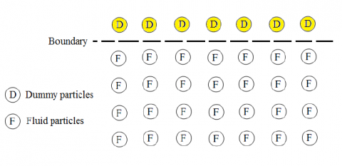
Applying boundary conditions is one of the key problems in Lagrangian and particle-based methods. Application of this method is usually more difficult in compared with the Eulerian and grid-based methods. This is due to the difference between the concept of position in two Eulerian and Lagrangian approaches. While in Eulerian approach the position is independent of time, it is a function of time in Lagrangian approach and defined with movement of material particles. In the present method, repulsive boundary conditions are used. The main purpose is preventing particles from crossing wall boundaries. Hence, a series of virtual solid particles are arranged around the fluid region. The virtual particles have a strong repulsive force which is proportional to inverse of distance between two particles. When a fluid particle enters the effective area of a virtual particle, dependent on the distance between them, this force is applied to the fluid particle along the line of centers of two particles. Repulsive force prevents fluid particle from closing to solid boundary and penetrating into the boundary. Fig 2 shows the arrangement of these particles for a wall and the force imposed by the particle is calculated as below [24]:
${{F}_{ij}}=\left\{ \begin{matrix} D\left[ {{\left( \frac{{{r}_{0}}}{{{r}_{ij}}} \right)}^{{{n}_{1}}}}-{{\left( \frac{{{r}_{0}}}{{{r}_{ij}}} \right)}^{{{n}_{2}}}} \right]\frac{{{x}_{ij}}}{r_{ij}^{2}} &\left( \frac{{{r}_{0}}}{{{r}_{ij}}} \right)\le 1 \\ 0 & \left( \frac{{{r}_{0}}}{{{r}_{ij}}} \right)>1 \\ \end{matrix} \right.$ (6)
where, n1, n2 and D are considered as 12, 6, and 0.01, respectively. r0 is the effect-distance of particle's force. Parameter r0 should be specified so that entering particles to solid region is prevented and it is usually in the order of the initial distance between main particles.
Figure 2. Arrangement of virtual particles for solid wall
It should be mentioned that the velocity of these particles is zero and their position is not updated. Density and pressure of these particles are also constant with time.
3.1 Conservation equations
The equations of mass and momentum govern the fluid flow and are expressed as follows:
$\frac{\text{1}}{\text{ }\!\!\rho\!\!\text{ }}\frac{\text{D }\!\!\rho\!\!\text{ }}{\text{Dt}}\text{+}\nabla \text{.}\,\vec{u}=0\,\,$ (7)
$\frac{D\vec{u}}{\text{Dt}}\text{=-}\frac{\text{1}}{\text{ }\!\!\rho\!\!\text{ }}\,\nabla \text{P+}\frac{\text{1}}{\text{ }\!\!\rho\!\!\text{ }}\nabla \text{.}\overset{\Rightarrow }{\mathop{\text{ }\!\!\tau\!\!\text{ }}}\,\,+\vec{g}$ (8)
In the above equation, ρ, u, τ indicate density, velocity filed and stress tensor, respectively. Also, g is the acceleration due to gravity.
3.2 Description of the equation of particles position
The equation of motion for particles at each time step is written as follows:
$\frac{d{{{\vec{r}}}_{a}}}{dt}={{\vec{u}}_{a}}$ (9)
When SPH method is applied to simulate the fluid flow, more modifications should be made. For example, instead of moving particles based on Eq. (9), motion of particles should be obtained using the following relation:
$\frac{d{{{\vec{r}}}_{a}}}{dt}={{\vec{u}}_{a}}\text{+}\varepsilon \sum\nolimits_{b}{{{m}_{b}}}\frac{{{{\vec{u}}}_{ba}}}{{{{\bar{\rho }}}_{ab}}}{{W}_{ab}}$ (10)
where ${{\bar{\rho }}_{ab}}=({{\rho }_{a}}+{{\rho }_{b}})/2$ and ${{\vec{u}}_{ba}}={{\vec{u}}_{b}}-{{\vec{u}}_{a}}$. ε is a constant $0\le \varepsilon \le 0.5$.Eq. (10) is regarded as the XSPH parameter and it is introduced by Monahan for the first time [25]. When particle-based methods are used for simulating fluid flows which are in contact with each other, XSPH parameter and modified expression for velocity are applied to prevent interference of particles. In addition, Eq. (10) guarantees that particles are moving with the velocity close to their nearby particles and for the relatively incompressible fluids like water, in the absence of viscosity, this keeps particles together in an ordered manner [26].
3.3. Description of the pressure state equation
A fluid like water is slightly compressible; but in most cases of fluid dynamics problems, it is approximated as an incompressible fluid. Another approach which is more consistent with SPH method is that fluid is treated as slightly compressible. This method, called weakly compressible smoothed particle hydrodynamics (WCSPH), is developed by applying weakly compressible condition using a state equation. This approach is an imitation of real fluid, but with small sound speed (to the extent that time steps are not very small) and, on the contrary, large enough to guarantee Much number M⁓0.1; therefore, density variations ∆ρ are smaller than 0.01ρ. The most common state equation utilized in SPH simulation with standard of weakly compressible condition is in the following form [19]:
$\text{P=B}\left[ {{\left( \frac{\text{ }\!\!\rho\!\!\text{ }}{{{\text{ }\!\!\rho\!\!\text{ }}_{\text{0}}}} \right)}^{\text{ }\!\!\gamma\!\!\text{ }}}\text{-1} \right]$ (11)
In the above equation, ρ0 is the reference density which for water is ρ0=1000kg/m3 and γ=7. The only modification required by state equation is changing the value of constant B. Sound speed in reference density is [13]:
${{\text{c}}^{\text{2}}}\text{=}\frac{\text{ }\!\!\gamma\!\!\text{ B}}{{{\text{ }\!\!\rho\!\!\text{ }}_{\text{0}}}}$ (12)
Therefore, if B=100ρ0u2/γ is selected, the considered density variation is less than 0.01. Here u is fluid velocity. Therefore, for obtaining B in each new problem, the maximum flow velocity should be estimated. A simple example is the problem of falling water column with the height of H. u2=2gH is an appropriate approximation in which, g is the Earth gravitational acceleration. According to this relation, speed of sound is calculated as c2=20gH.
3.4 Description of non-Newtonian model
For modeling problem, sand is regarded as a non-Newtonian fluid, by Bingham plastic model. This kind of fluids can sustain a specific amount of stress (yield stress) without flowing. Obviously, in higher values than yield stress, the fluid continuously introduces strain. The stress relation in this model is as follows [20]:
${{\mu }_{eff}}={{\mu }_{B}}+\frac{{{\tau }_{B}}}{{\dot{\gamma }}}$ (13)
In which μB is viscosity coefficient, τB is Bingham yield stress. ${\dot{\gamma }}$ also demonstrates shear strain rate and it is defined as:
$\dot{\gamma }\text{=}\sqrt{2{{\left( \frac{\partial u}{\partial x} \right)}^{2}}+2{{\left( \frac{\partial v}{\partial y} \right)}^{2}}+{{\left( \frac{\partial u}{\partial x}+\frac{\partial v}{\partial y} \right)}^{2}}}$ (14)
where parameters u and v are velocity vectors.
For validation and being sure about the applied algorithm, the current solution method is used for three different problems.
4.1 Validating flow through submerged hatch
As the first simulation, using the current numerical method, the outlet flow through submerged hatch is modeled and VOF method according to reference [21] is considered for validation. As the initial geometry of problem, the reservoir length and the initial water height are both considered to be 0.15 m and hatch height to be 0.035 m. In the first moment, it is assumed that the hatch is opened abruptly. Regarding the convergence criteria, time step is considered to be 0.001 s and locative interval to be 0.005. Computational properties in the current method are shown in Table 1. The conditions of reservoir free surface and the outlet flow through hatch at different times are shown in Figure 3 based on the mentioned methods.
Table 1. The computational properties in the problem of passing flow through submerged hatch
|
Water particles |
900 |
|
Wall particles |
1036 |
|
Total particles |
1236 |
|
Initial particle distance |
0.005 m |
|
Time step |
0.001 s |
Considering Figure 3, very good agreement for specifying conditions of water surface in reservoir and in outlet of hatch is observed between two methods.
As the last problem of this chapter, the outlet flow from orifice was modeled and validated. According to reference [13], the orifice opening in the height of 0.055 m is 0.045 m from the ground. In Figure 4, the variation of fluid free surface at 0.14 s after opening hatch is shown.
As it is seen in this figure, there is a very appropriate agreement among the results of numerical method of VOF and WCSPH method.
4.2 Simulation of classic dam failure problem
Another simulation performed for validating the computational algorithm is the classical model of dam failure problem during which the results of current simulation are compared with experimental ones obtained by Ozmen and Kocaman [14]. In this process, validation is performed by an experimental model. In numerical calculations, the upper boundary is wall reminding that no flow enters the reservoirs and the reservoir length is constant. The lower boundary for dry-bed experiment is treated as outlet flow; but in wet-bed experiment this is applied as wall because of closing with vertical metal plate (end of reservoir). Below boundary (bottom) is also considered as closed and above boundary (water surface) as symmetric for atmospheric pressure values on surface.
Figure 3. The water surface profile in reservoir and outlet of hatch obtained by WCSPH and VOF methods [21] at a) t=0 s, b) t=0.04 s, c) t=0.1, and d) t=0.14 s
Figure 4. Variations of water surface at 0.14 s after opening orifice. Comparison between present results and the one of Ref. [21]
In Table 2, the properties corresponding to initial dimensions and computational parameters for simulating dam failure problem and comparing with experimental model can be observed. Based on this model, initial geometry of dam failure is drawn in Figure 5, which the initial depth of upstream water is h0=25 cm and that of downstream water is variable. In this model, length of reservoir d=9cm and height of reservoir is H=26cm. Lengths of upstream and downstream are 4.65 cm and 4.35 cm respectively to be consistent with experimental model.
Table 2. Computational parameters in dam failure problem
|
Water particle |
7740 |
|
Wall particle |
2088 |
|
Total particle |
9528 |
|
Smoothing length (h) |
1.5L0 |
|
XSPH factor |
0.1 |
|
Upstream height |
0.25m |
|
Initial particle distance |
0.0125m |
|
Time step |
0.0001s |
Figure 5. Dimensions and properties of dam failure model
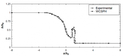
In Figures 6-11, flow depth (h) and horizontal length (x) are non-dimensionalized by initial depth of upstream (h0). Time (t) is also applied in the form of the dimensionless parameter $T=t(g/h_0)^{0.5}$. Parameter α introduces the ratio of height of downstream to that of upstream whose values for three different simulations are 0, 0.1 and 0.4 respectively. In these figures qualitative changes of water surface level and the created wave by dam failure are compared and validated by results of experimental model of Ref. [22].
Figure 6. Comparison between results of simulation by WCSPH model and experimental model [22]. Free surface profile along initial states of dam failure at non-dimensional time of T=1.13 for dry bed with α=0
Figure 7. Comparison between results of simulation by WCSPH model and experimental model [22]. Free surface profile along initial states of dam failure at non-dimensional time of T=2.76 for dry bed with α=0
Figure 8. Comparison between results of simulation by WCSPH model and experimental model. Free surface profile along initial states of dam failure at non-dimensional time of T=1.57 for dry bed with α=0.1
Figure 9. Comparison between results of simulation by WCSPH model and experimental model [22]. Free surface profile along initial states of dam failure at non-dimensional time of T=2.38 for dry bed with α=0.1
Figure 10. Comparison between results of simulation by WCSPH model and experimental model [22]. Free surface profile along initial states of dam failure at non-dimensional time of T=1.50 for dry bed with α=0.4
Figure 11. Comparison between results of simulation by WCSPH model and experimental model [22]. Free surface profile along initial states of dam failure at non-dimensional time of T=2.38 for dry bed with α=0.4
Considering the obtained results, variations of free surface profile and the front of created wave by dam failure can be observed during time. The results show a good qualitative agreement among the results of numerical and experimental model. In the manner that for the model corresponding to dry upstream, the results of WCSPH and experimental models are so close to each other which can be hardly distinguished. The dynamic nature of particles in SPH method can be regarded as the reason of this behavior which regarding to this nature, particles harbor turbulence in themselves.
4.3. Validation of water-sediment two-phase flow caused by dam failure on erodible bed
Dam failure on erodible bed causes transportation of sediments behind the dam reservoir and abrupt changes of bed. Nature and behavior of solid-liquid two-phase flows are different with those of single-phase flows. Investigation of velocity and behavior of these flows is complicated due to existence of suspending and depositable particles and they always attract the attention of researchers because of their wide applications in industry. One of the most complicated problems in simulation of two-phase flows is existing huge density difference among available phases. In this section, the suggested model for simulating the flow caused by dam failure on erodible bed and investigating the morphological processes mechanism is described. For this purpose, the physical model of Ref. [23] is regarded for simulation and analysis. Accurate specification of different effective parameters on the properties of two-phase flows has considerable importance. For simulating sediments, non-Newtonian Bingham plastic model is utilized which the reason of its application has been already assessed. Yield stress and effective Bingham viscosity are among the effective parameters for simulation. In this simulation, according to experimental relations, the value of yield Bingham stress τy is considered τB=0.447Pa [24]. In addition, Bingham plastic viscosity is equal to μ=0.04Pa.s. The geometrical and rheological values used for simulation of the current problem are reported in Tables 3 and 4.
Table 3. The geometrical properties of the water-sediment simulation model
|
Water column width |
1m |
|
Sediment column width |
2.5m |
|
Water column height |
0.05m |
|
Sediment column height |
0.1m |
|
XSPH factor |
0.07m |
|
Initial particle distance |
0.05m |
|
Time step |
0.00003m |
Table 4. The rheological properties of the water-sediment simulation model
|
Yield stress |
0.447Pa |
|
Water viscosity |
0.001Pa.s |
|
Sediment viscosity |
0.04Pa.s |
|
Water density |
1000kg/m3 |
|
Sediment density |
1940kg/m3 |
Figure 12. The initial geometry of water-sediment in simulation model
Figure 13. The initial geometry of water-sediment in experimental model
In Figure 12 the initial simulation geometry and in Figure 13 the experimental model of the water-sediment two-phase flow created by dam failure on erodible bed are demonstrated in which the upper flow introduces water and the below one introduces sediment.
Figure 14. Investigating the progress of wave front, sediment transport, and free surface at t=0.25s between experimental model (above figure) and the current work (below figure)
Figure 15. Investigating the progress of wave front, sediment transport, and free surface at t=0. 5s between experimental model (above figure) and the current work (below figure)
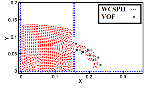
In Figures 14-16, using the current method, the results of modeling free surface profile are investigated at different times. In these figures, the experimental results and the ones obtained by the current method are shown. Regarding the lack of accurate dimensions and sizes in experimental results and also available different interpretations, qualitative comparison is regarded in this section. By observing the results, the trend of progressing flood created by dam failure demonstrates that in the beginning of this process an intensely dense wave develops through the downstream causing dramatic increase in water depth. The initial wave energy causes considerable erosion at the beginning of bed. During the time, the initial wave transports the leached particles of bed to a distance in downstream. Therefore, by decreasing the wave energy and also increasing the difference in bed profile, sediments are deposited. As this wave spreads through downstream, it wanes gradually. Progress of the initially created wave also decreases water level in upstream.
Figure 16. Investigating the progress of wave front, sediment transport, and free surface at t=0.75s between experimental model (above figure) and the current work (below figure)
After validation of algorithm for different models, it has applied to simulate Sand beach. The computational parameters utilized for simulating this flow, including water properties (Newtonian viscous fluid) and those of sand (non-Newtonian Bingham model fluid) are brought in Table 5.
Table 5. The computational parameters for beach flow simulation
|
Sand density |
1950 kg/m3 |
|
Water density |
1000 kg/m3 |
|
Total particles |
6471 |
|
Initial particle distances |
0.04m |
|
Time steps |
0.00002s |
After introducing computational parameters, properties of water and sand are the only properties required for modeling. A rheological model is used for describing the behavior of sand. In other words, sand is regarded as a Bingham plastic fluid [25, 26]. As it is mentioned before, in stresses less than yield stress, Bingham fluid does not introduce any strain but in values higher than yield stress, its internal structure distorts and shear movement becomes possible. On condition that shear stress is less than yield stress, internal structure establishes again. In non-Newtonian fluid like Bingham, unlike Newtonian fluid, viscous coefficient changes dependent on strain rate. The values of yield stress and viscous coefficient of the Bingham fluid for modeling sand is according to Ref. [20] which are selected after try and error to have the best values for our studied sand. Reminding that two kinds of sand are studied, different values for yield stress τB=200Pa and τB=1000Pa with constant μB=0.1N.s/m2 and ρsand=1950kg/m3 are considered for two types of beds whose physical properties are consistent with experiments of Rzadkiewicz et al. [27].
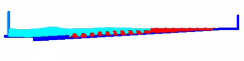
The modeling results for non-Newtonian fluid of sand with τB=200Pa and μB=0.1N.s/m2 in different time intervals are available in Figs. 17-21. The demonstrated regions from coastal profile include the area before and after wave break to reflect its effect, if available, on changing bed profile. According to the result, modeled bed under the effect of finite yield stress of τB=200Pa varies fast and after 2 to 4 seconds (dependent on conditions of simulation), the profile of ripples become steady.
Figure 17. The variations of first type of sandy coast bed in t=0
Figure 18. The variations of first type of sandy coast bed in t=0.7s
Figure 19. The variations of first type of sandy coast bed in t=2s
Figure 20. The variations of first type of sandy coast bed in t=4s
Figure 21. The variations of first type of sandy coast bed in t=8s
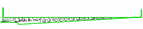
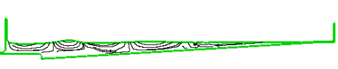
For next step, streamline contours have shown in Figures 22-27. According to the results, streamline contours has irregularity in early moments. But in the following, regular structure occurs with progress in time and wave formation.
Figure 22. The streamline contour of first type of sandy coast bed in t=0.7
Figure 23. The streamline contour of first type of sandy coast bed in t=4
Figure 24. The streamline contour of first type of sandy coast bed in t=8
Figure 25. The streamline contour of first type of sandy coast bed in t=10
Figure 26. The streamline contour of first type of sandy coast bed in t=12
Figure 27. The streamline contour of first type of sandy coast bed in t=16
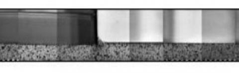
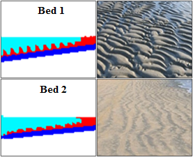
Figure 28. Comparison between two kinds of modelled beds possessing different yield stresses (left hand side) and comparison between these two models with their similar real sandy beds (right hand side)
Two types of costal beds which are defined and distinguished from each other by their difference in value of yield stress are shown in Figure 28. Modeling the effect of wave in these two beds (left hand side) and the figures of similar real beds to this modeling (right hand side) are shown.
In this study sandy, coast bed was investigated with WCSPH method as the main model. To validate this method, the different fluidic phenomena were simulated. During this step, the problems of outlet flow through a hatch and the phenomenon of dam failure in two cases of wet and dry beds as the Newtonian events and the problem of water-sediment two-phase flow as a non-Newtonian fluidic phenomenon are considered for simulation and validation during which the investigation proves the correctness of simulation and desired accuracy of current method. As the main model, changes in profile of a sandy coast bed with specific physical and rheological properties were modeled at different times under the effect of a sinusoidal wave maker pedal. The appearance of modeled bed under the effect of finite yield stress of τB=200 Pa varies fast and after 2 to 4 seconds (dependent on conditions of simulation), the profile of ripples become steady. In addition, since the second type of bed includes finer particles, a significant change in profile cannot be observed; but on the contrary, for the first type of bed by considering more finite yield stress, the resulted change of profile is observable. The dentate profile appearance of this type of beds is ripple-shaped which is among the most important and common profile changes in sandy beds.
|
D |
Repulsive force parameter |
|
g |
Gravity constant (m/s2) |
|
h |
Smoothing length (m) |
|
L0 |
Initial particle distance(m) |
|
m |
Mass (kg) |
|
P |
Pressure (Pa) |
|
r |
Position vector (m) |
|
t |
Time (s) |
|
T |
Non dimensional time (s) |
|
u,v |
Horizontal velocity, Vertical velocity (m/s) |
|
Greek symbols |
|
|
α |
Upstream to downstream ratio |
|
$\dot{\gamma}$ |
Shear strain rate (s-1) |
|
ε |
XSPH factor |
|
µ |
Viscosity ($N.s/{{m}^{2}}$) |
|
µeff |
Effective viscosity ($N.s/{{m}^{2}}$) |
|
ρ |
Density ($\text{kg/}{{\text{m}}^{\text{3}}}$) |
|
τ |
Shear stress (Pa) |
|
τB |
Yield (Pa) |
[1] Goodarzi Z, Ahmadi NA, Bayareh M. (2018). Numerical investigation of off-centre binary collision of droplets in a horizontal channel. Journal of the Brazilian Society of Mechanical Sciences and Engineering 40: 1-10. http://dx.doi.org/10.1007/s40430-018-1075-y
[2] Hassanzadeh M, Ahmadi NA, Bayareh M. (2019). Numerical simulation of the head-on collision of two drops in a vertical channel. Journal of the Brazilian Society of Mechanical Sciences and Engineering 41: 1-14. http://dx.doi.org/10.1007/s40430-019-1624-z
[3] Bayareh M, Mortazavi S. (2009). Geometry effects on the interaction of two equal-sized drops in simple shear flow at finite Reynolds numbers. 5th international conference: Computational methods in multiphase flow, WIT Transactions on Engineering Sciences 63: 379-388.
[4] Bayareh M, Mortazavi S. (2013). Equilibrium position of a buoyant drop in couette and poiseuille flows at finite reynolds numbers. Journal of Mechanics 20: 53-58. http://dx.doi.org/10.1017/jmech.2012.109
[5] Bayareh M, Mortazavi S. (2011). Binary collision of drops in simple shear flow at finite Reynolds numbers. Advances in Engineering Software 42: 604-611. http://dx.doi.org/10.1016/j.advengsoft.2011.04.010
[6] Bayareh M, Mortazavi S. (2011). Migration of a drop in simple shear flow at finite Reynolds numbers: Size and viscosity ratio effects. Proceeding of International Conference on Mechanical, Industrial, and Manufacturing Engineering (ICMIME).
[7] Armandoost P, Bayareh M, Ahmadi NA. (2018). Study of the motion of a spheroidal drop in a linear shear flow. Journal of Mechanical Science and Technology 32: 2059-2067. http://dx.doi.org/10.1007/s12206-018-0415-2
[8] Mohammadi MS, Bayareh M, Ahmadi NA. (2019). Pairwise interaction of drops in shear-thinning inelastic fluids. Korea-Australia Rheology Journal 31: 25-34. http://dx.doi.org/10.1007/s13367-019-0003-8
[9] Liu GR, Gu YT. (2005). An introduction to meshfree methods and their programming. Springer.
[10] Monaghan JJ, Gingold RA. (1983). Shock simulation by the particle method SPH. Journal of Computational Physics 52: 374-389. http://dx.doi.org/10.1016/0021-9991(83)90036-0
[11] Hu XY, Adams NA. (2007). An incompressible multi-phase SPH method. Journal of Computational Physics 227: 264-278.
http://dx.doi.org/10.1016/j.jcp.2007.07.013
[12] Khayyar A, Gotoh H, Shao SD. (2008). Corrected incompressible SPH method for accurate water-surface tracking in breaking waves. Coastal Engineering 55: 236-250. http://dx.doi.org/10.1016/j.coastaleng.2007.10.001
[13] Khayyer A, Gotoh H, Shao S.) 2009). Enhanced predictions of wave impact pressure by improved incompressible SPH methods. Applied Ocean Research 31: 111-131. http://dx.doi.org/10.1016/j.apor.2009.06.003
[14] Rogers BD, Dalrymple RA, Stansby PK. (2010). Simulation of caisson breakwater movement using 2-D SPH. Journal of Hydraulic Research 48: 135-141. http://dx.doi.org/10.1080/00221686.2010.9641254
[15] Lind SJ, Stansby PK, Rogers BD. (2016). Incompressible–compressible flows with a transient discontinuous interface using smoothed particle hydrodynamics (SPH). Journal of Computational Physics 309: 129-147. http://dx.doi.org/10.1016/j.jcp.2015.12.005
[16] Ellero M, Kröger M, Hess S. (2002). Viscoelastic flows studied by smoothed particle dynamics. Journal of Non-Newtonian Fluid Mechanics 105: 35-51. http://dx.doi.org/10.1016/S0377-0257(02)00059-9
[17] Shao S, Lo EYM. (2003). Incompressible SPH method for simulating Newtonian and non-Newtonian flows with a free surface. Advances in Water Resources 26: 787-800. http://dx.doi.org/10.1016/S0309-1708(03)00030-7
[18] Violeau D, Rogers BD. (2016). Smoothed particle hydrodynamics (SPH) for free-surface flows: Past, present and future. Journal of Hydraulic Research 54: 1-26. http://dx.doi.org/10.1080/00221686.2015.1119209
[19] Abdekerem X, Wang L, Jin A, Geni M. (2014). Numerical modeling and simulation of wind blown sand morphology under complex wind-flow field. Journal of Applied Mathematics 2014: 1-11. http://dx.doi.org/10.1155/2014/590358
[20] Ablimit A, Geni M, Xu Z, Tursun M, Abdikerem X. (2011). Numerical study on Aeolian sand ripples forming and moving process in desert highway. Key Engineering Materials 462: 1032-1037. http://dx.doi.org/10.4028/www.scientific.net/KEM.462-463.1032
[21] Finn J, Li M, Apte SV. (2016). Particle based modeling and simulation of natural sand dynamics in the wave bottom boundary layer. Journal of Fluid Mechanics 796: 340-385. http://dx.doi.org/10.1017/jfm.2016.246
[22] Morris JP, Fox PJ, Zhu Y. (1997). Modeling low reynolds number incompressible flows using SPH. Journal of Computational Physics 136: 214-226. http://dx.doi.org/10.1006/jcph.1997.5776
[23] Monaghan JJ. (1985). Extrapolating B splines for interpolation. Journal of Computational Physics 60: 253-262. http://dx.doi.org/10.1016/0021-9991(85)90006-3
[24] Hirt CW, Amsden AA, Cook JL. (1974). An arbitrary Lagrangian-Eulerian computing method for all flow speeds. Journal of Computational Physics 14: 227-253. http://dx.doi.org/10.1016/0021-9991(74)90051-5
[25] Monaghan JJ. (1989). On the problem of penetration in particle methods. Journal of Computational physics 82: 1-15. http://dx.doi.org/10.1016/0021-9991(89)90032-6
[26] Molteni D, Colagrossi A. (2009). A simple procedure to improve the pressure evaluation in hydrodynamic context using the SPH. Computer Physics Communications 180: 861-872. http://dx.doi.org/10.1016/j.cpc.2008.12.004
[27] Brebbia CA, Benassai G, Rodríguez G. (2009). Coastal processes. WIT Press.